1. Antenna Overview
This page shows the modelled radiation behaviour of the Boscastle long-wire – a single continuous end-fed wire, roughly 4 m above ground, routed around the garden to make the most of the available space in an Area of Outstanding Natural Beauty.
For the Boscastle installation, the wire is broken into several straight segments with bends that approximate the real-world layout. Each segment was translated into NEC geometry and simulated over real ground using xnec2c, then re-processed in Python to give 2D cuts, low-angle gain estimates and fully rotatable 3D plots.
The yellow line marks the +Y / North direction. The Z axis points upwards. The faint grey ring is the ground plane (z = 0). Lobes pointing along the yellow arrow are radiating north; opposite is south.
Key modelling assumptions:
- NEC2 real ground with typical damp-soil conductivity.
- Far-field patterns sampled from 0°–90° elevation and all azimuths.
- Total gain in dBi; patterns normalised on a per-plot basis for clarity.
- Direction of true North aligned to local map orientation in the model.
The goal here is to understand relative directionality and launch angles by band, rather than claim absolute gain figures at the station.
2. Low-Angle DX Potential by Band
The first summary is a rough comparison of low-angle gain around 20° elevation for each HF/VHF band. This is where most long-haul DX F-layer signals tend to arrive.
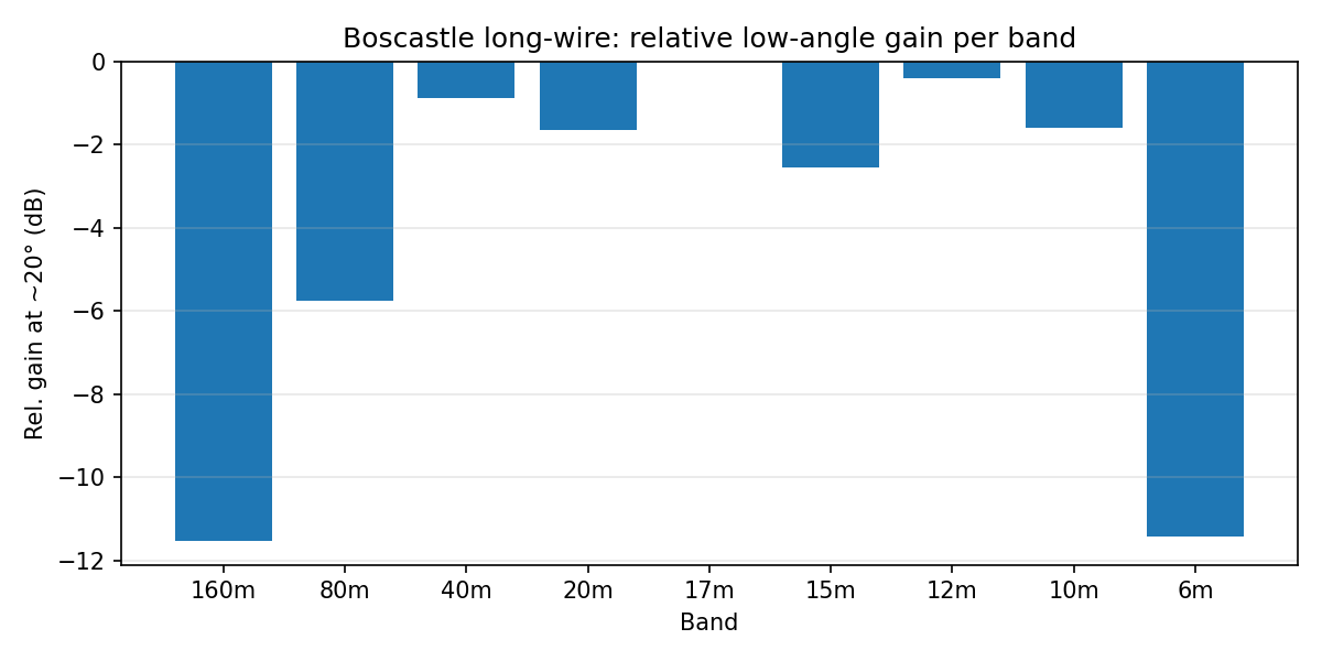
In this model the higher HF bands generally have the best low-angle performance from Boscastle, with 17 m–12 m looking particularly promising for DX. 160 m and 6 m are more compromised at low angles, which matches the “sounds great locally, harder to reach true DX” experience on those bands.
3. 2D Azimuth & Elevation Cuts
The next graphic shows classic 2D cuts: azimuth patterns at a fixed low elevation, and elevation cuts through the strongest horizontal directions, for each amateur band from 160 m to 6 m.
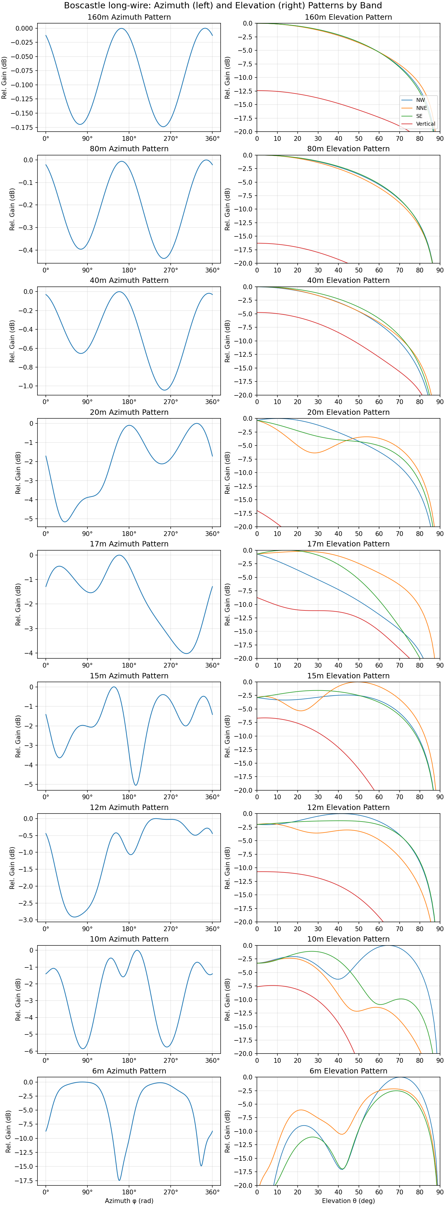
At lower bands you can see strong high-angle lobes suitable for near-vertical incidence skywave (NVIS) around the UK. As frequency increases, additional azimuth lobes appear and the first nulls drop to lower elevation angles, sharpening the primary DX directions.
4. Interactive 3D Radiation Patterns (All Bands)
This interactive view lets you rotate, zoom and inspect the full 3D pattern for each band. Use the dropdown to select the band, then drag to rotate and scroll to zoom. Hover over the surface for numeric gain read-outs.
Remember: the yellow arrow points to North, and the grey ring indicates the ground plane. In the Boscastle layout the longest leg of the wire runs roughly NW–SE, so you’ll see stronger lobes favouring those quadrants on many bands – which tallies nicely with WSPR/FT8 spots that favour Scandinavia, eastern Europe and long-path Pacific on a good day.
5. Per-Band Interactive DX Band Cards
These interactive “DX Band Cards” combine three views:
- DX summary panel — best lobe direction, take-off angle, and a low-angle “DX score”.
- Azimuth × elevation heatmap — colours show relative far-field gain (0 dB = strongest point on that band).
- Low-angle gain comparison — how that band compares to all others at ~20° take-off (typical DX angle).
These plots are generated from boscastle_fullpattern.csv and reflect the real NEC2 simulation of the Boscastle long-wire geometry.
160 m Band Interactive Card
80 m Band Interactive Card
40 m Band Interactive Card
20 m Band Interactive Card
17 m Band Interactive Card
15 m Band Interactive Card
12 m Band Interactive Card
10 m Band Interactive Card
6 m Band Interactive Card
Each interactive card lets you explore the radiation behaviour of the Boscastle long-wire at a specific amateur band:
- Heatmap — the best DX directions appear as bright warm colours. Cooler colours show weaker gain.
- Vertical “best heading” line — where the antenna is strongest at low angles.
- ~20° DX ring — indicates typical long-distance F-layer launch angle.
- DX score — a simplified, relative estimate of real-world DX performance on that band for this antenna geometry.
6. Real QSOs vs NEC Predictions
The NEC2 patterns above tell us what the Boscastle long-wire should do in free space plus ground. Here we compare that with what actually happened on air, using logged QSOs and derived take-off angles.
All of these diagnostics are generated from a merged QSO dataset (qso_takeoff_angles_enriched.csv) and the same NEC far-field export used elsewhere (boscastle_fullpattern.csv).
Overall NEC vs QSO take-off angle correlation (all bands)
Each point is a QSO. The horizontal axis is the NEC-predicted low-angle peak for that band; the vertical axis is the QSO-derived take-off angle from the hop geometry. Points fall into vertical stripes (one per band), forming a broad cloud between roughly 5° and 25° elevation. The diagonal line marks perfect agreement; the low Pearson correlation confirms that NEC gives a sensible DX window rather than an exact angle for each individual contact.
6.1 Per-band azimuth performance – NEC vs local + DX QSOs
These plots combine the NEC low-angle azimuth gain with QSO bearing histograms. The solid curve is NEC relative gain averaged over a 5°–25° elevation window; the filled bars show where the local (< 3000 km) and DX (≥ 3000 km) QSOs actually came from in azimuth.
160 m — NEC low-angle gain vs local & DX QSO bearings
On 160 m the pattern is dominated by near-vertical skywave and ground losses. Any alignment between NEC lobes and QSO clusters is a bonus rather than a guarantee, but deep nulls with very few QSOs still flag genuine dead directions.
80 m — NEC low-angle gain vs local & DX QSO bearings
80 m shows the classic split between European NVIS and longer single-hop DX. Where the DX histogram peaks line up with NEC low-angle lobes, the Boscastle wire is punching out nicely; quiet azimuths that coincide with NEC nulls are genuinely hard directions for night-time DX.
40 m — NEC low-angle gain vs local & DX QSO bearings
On 40 m the NEC lobes begin to narrow and the DX-bearing histogram follows them closely. This is a good sanity check that both the model geometry and the QSO great-circle bearings are behaving as expected.
20 m — NEC low-angle gain vs local & DX QSO bearings
On 20 m, the low-angle NEC pattern lines up well with the measured QSO bearings. DX contacts mostly follow the strongest modelled lobes at shallow elevation, while local and regional QSOs tend to sit under the weaker side-lobes. Overall, the azimuth distribution is more selective than on 40 m but still broad enough to cover the main great-circle corridors actually worked in the log
17 m — NEC low-angle gain vs local & DX QSO bearings
17 m is a nice mid-HF case: NEC shows a few strong low-angle lobes, and the DX QSO density piles up exactly there. Sparse bins in between the lobes show where Boscastle is relatively deaf on this band.
15 m — NEC low-angle gain vs local & DX QSO bearings
On 15 m the antenna becomes more directional. The DX histogram tends to “sit” on one or two main NEC lobes, with quiet regions elsewhere. That matches real-world experience of 15 m being very good into some quadrants and stubbornly poor into others.
12 m — NEC low-angle gain vs local & DX QSO bearings
12 m shows strong selectivity: most DX QSOs fall into a few favoured headings that coincide with NEC lobes. Gaps where both NEC gain and QSO counts are low are directions where the Boscastle long-wire simply isn’t a great radiator on this band.
10 m — NEC low-angle gain vs local & DX QSO bearings
On 10 m the pattern is very lumpy: sharp NEC lobes and deep nulls. The QSO bearings hug those lobes when the band is open, giving a good visual explanation of why some 10 m paths from Boscastle are spectacular while others are almost impossible.
6 m — NEC low-angle gain vs local & DX QSO bearings
6 m is heavily Es- and scatter-driven, so the QSO histogram is more stochastic, but you can still see a preference for headings where the NEC model has usable low-angle gain.
6.2 Per-band 2D pattern vs QSO footprint
These plots show the NEC azimuth × elevation pattern as a coloured heatmap, with individual QSOs overlaid as points. Warm colours = stronger NEC gain; cooler colours = weaker. QSO markers are positioned at their bearing and inferred take-off angle, so you can see which parts of the pattern are actually being “used” on air.
160 m: pattern vs QSO footprint
80 m: pattern vs QSO footprint
40 m: pattern vs QSO footprint
20 m: pattern vs QSO footprint
17 m: pattern vs QSO footprint
Here you can see the DX contacts clustering in the bright low-angle lobes, with fewer QSOs in the cool-coloured nulls. The vertical axis is elevation (0° at the centre, 90° at the outer ring), so the DX cluster sits in the ~10–25° annulus.
15 m: pattern vs QSO footprint
12 m: pattern vs QSO footprint
10 m: pattern vs QSO footprint
6 m: pattern vs QSO footprint
7. Data & Modelling Notes
All of the plots on this page are derived from a single NEC2 far-field export: boscastle_fullpattern.csv, containing total gain versus phi (azimuth), theta (elevation) and frequency. A small Python toolkit was used to:
- parse the CSV and split it by amateur band,
- normalise and re-sample the patterns onto regular angle grids,
- generate 2D azimuth/elevation cuts, and
- convert the spherical data to Cartesian coordinates for the 3D Plotly views.
Example CSV header (boscastle_fullpattern.csv)
mhz,phi,theta,gain_total,gain_horiz,gain_vert,gain_rhcp,gain_lhcp
1.900000,0,0,-5.96,-6.22,-18.38,-8.97,-8.97
1.900000,0,1.0,-5.96,-6.22,-18.39,-8.97,-8.97
1.900000,0,2.0,-5.97,-6.23,-18.39,-8.98,-8.97
...
The scripts themselves live alongside the NEC data as plot_boscastle_3d_plotly.py and plot_boscastle_3d_plotly_multiband.py, and run inside a dedicated virtual environment so they don’t disturb any other radio-related Python experiments on the system.