WSPR Take-off Angles — M7SQI

What the viewer showed

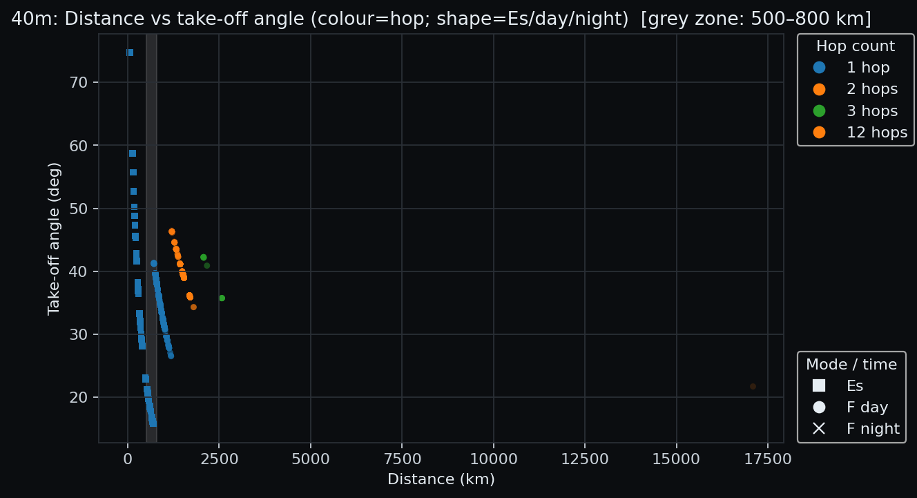
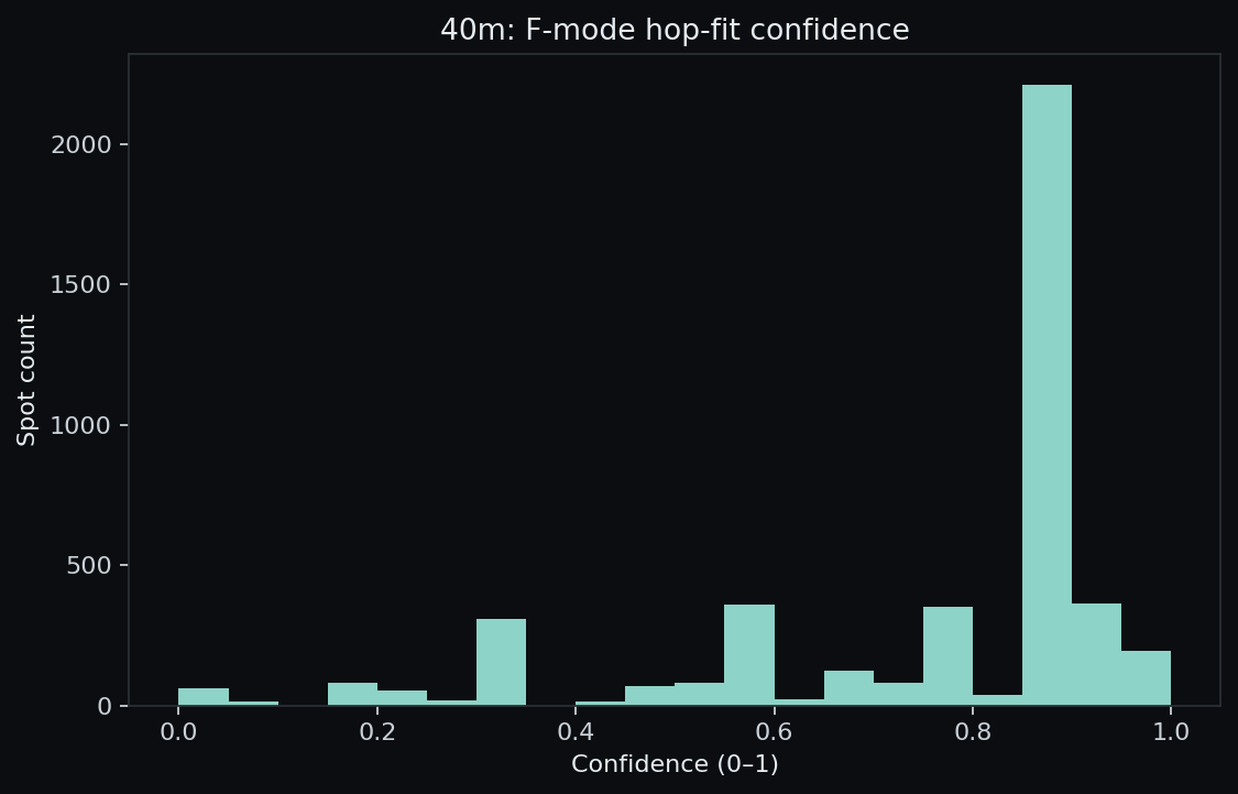
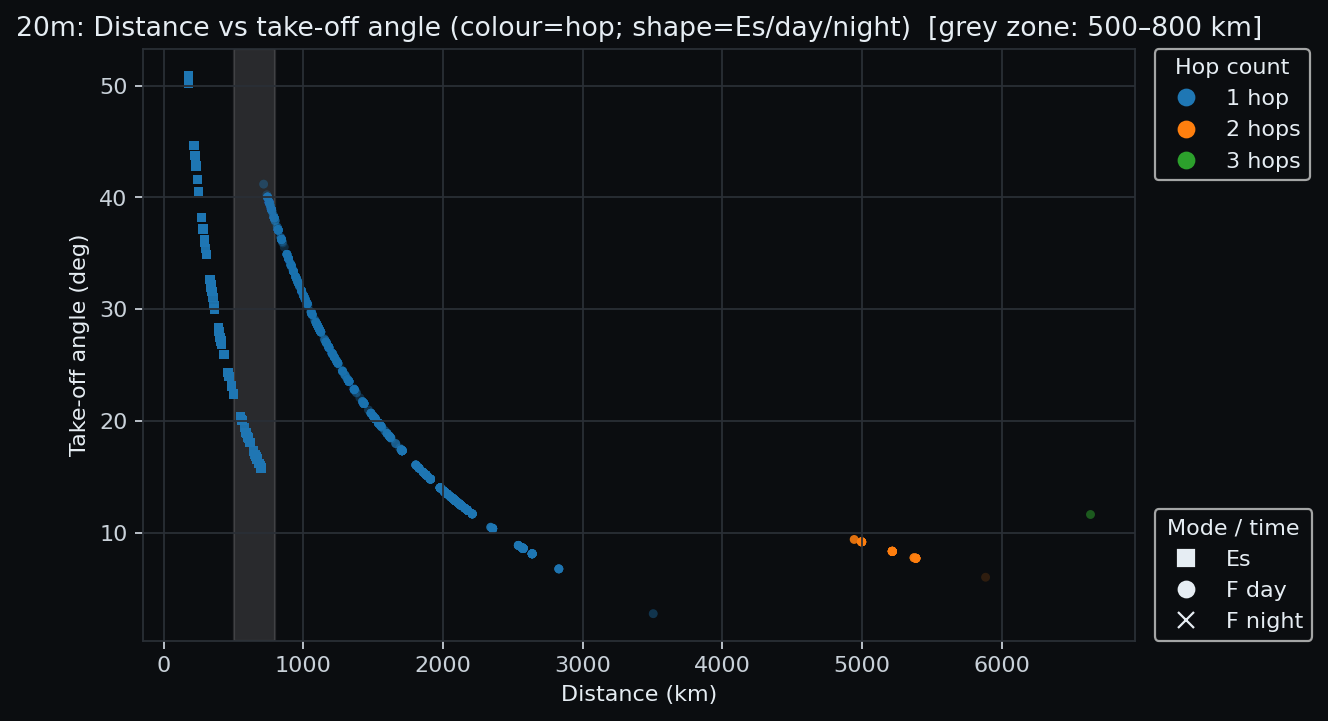
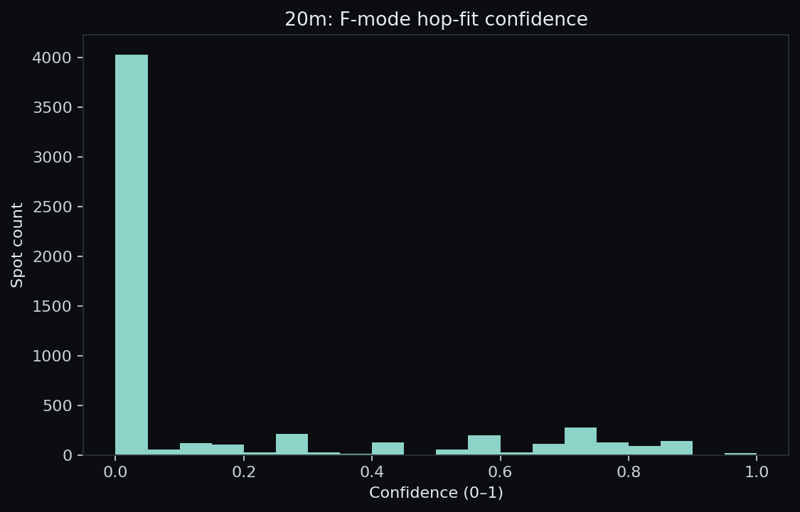
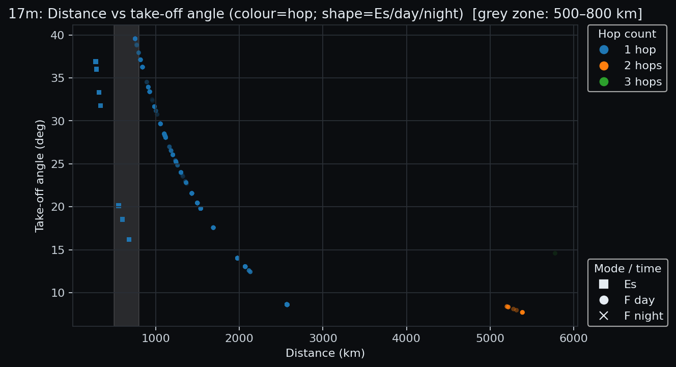
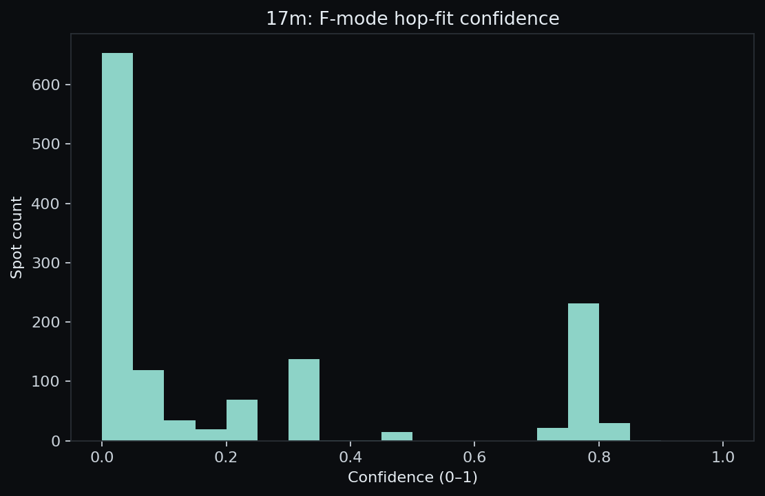
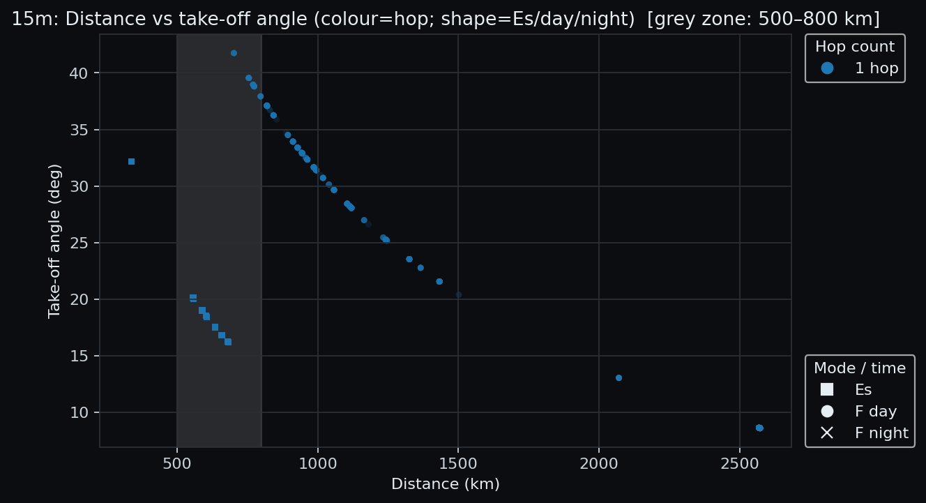
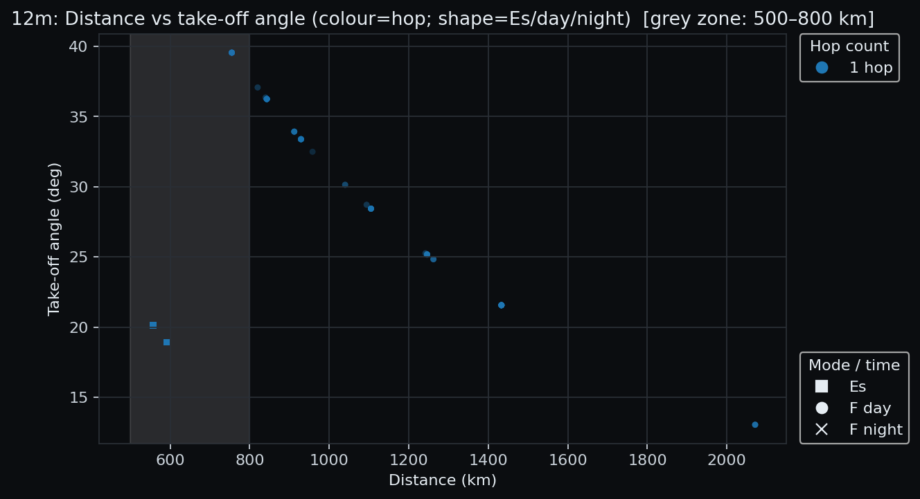
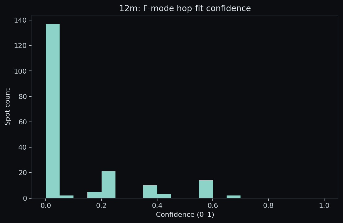
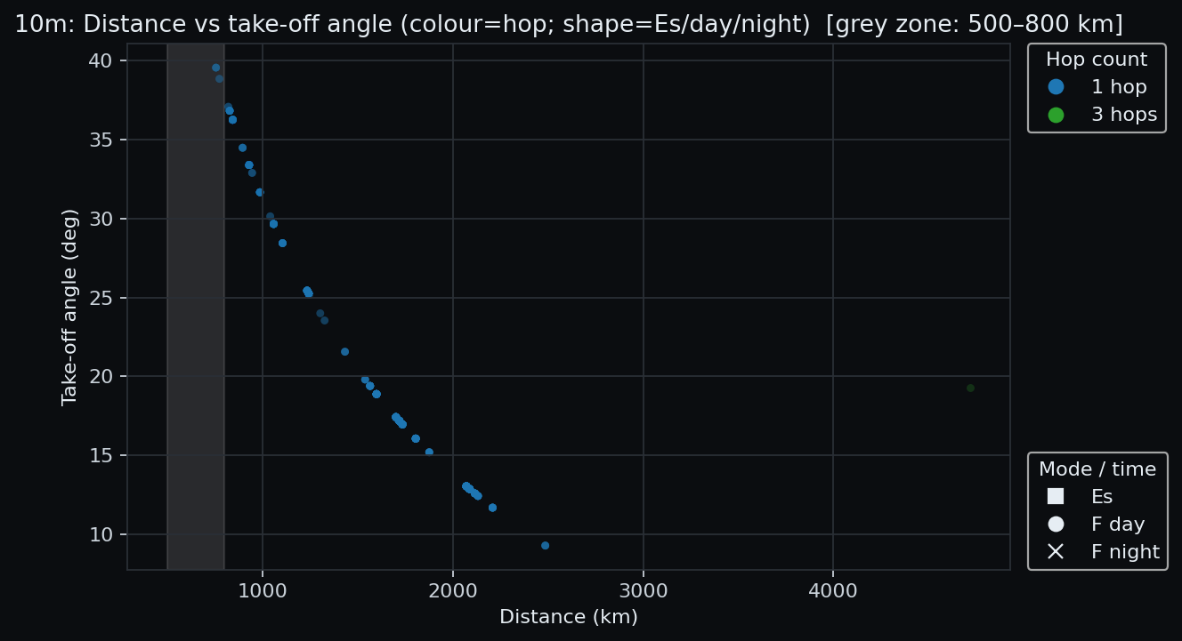
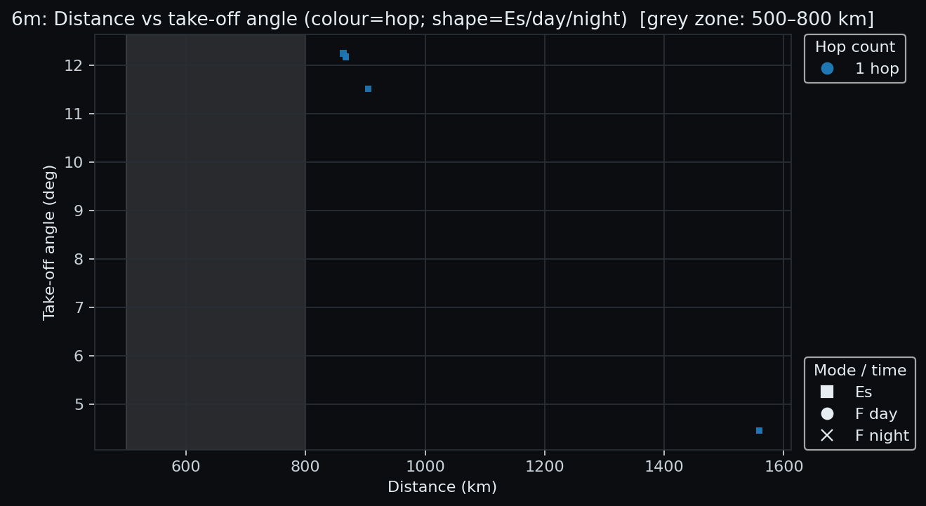
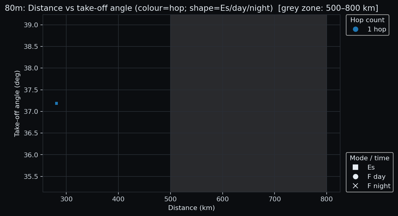
Each point represented a WSPR spot. From the great-circle distance, a take-off angle (TX elevation) was inferred by assuming ionospheric “mirror” hops at a virtual height. Colours encoded the inferred hop count; shapes indicated propagation/time: ■ Es, ● F (day), × F (night). Point opacity reflected fit confidence. A light grey vertical band marked the Es–F overlap region (where classification was less certain).

How the angles were calculated (ham-science summary)

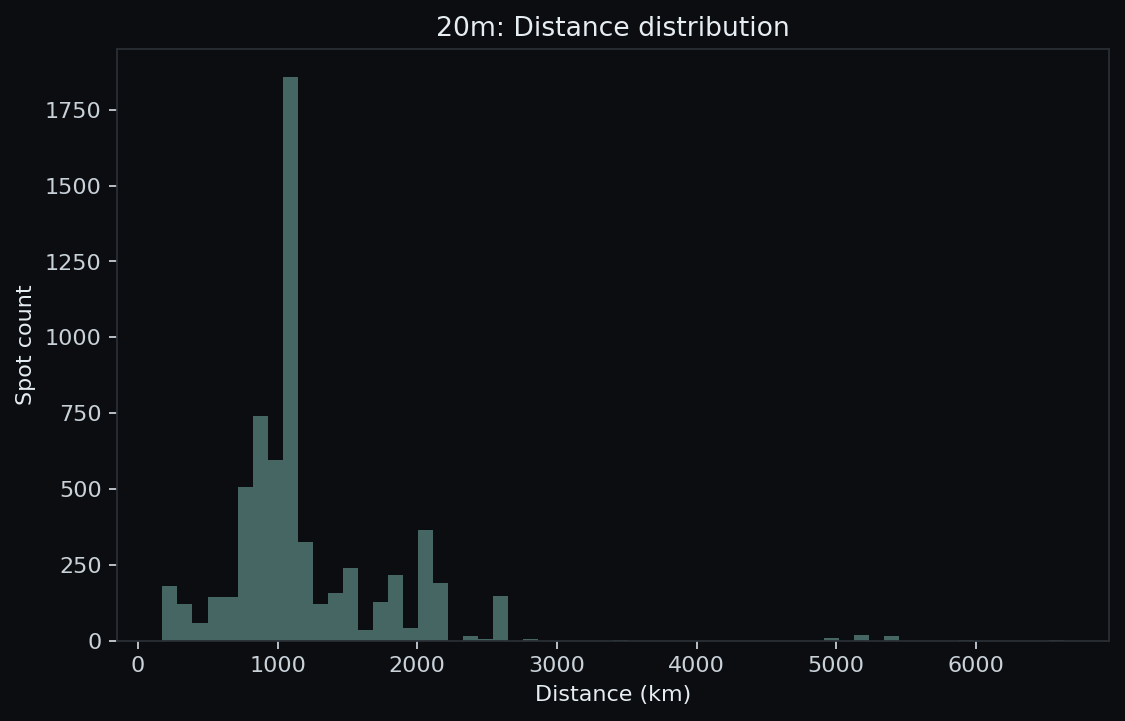
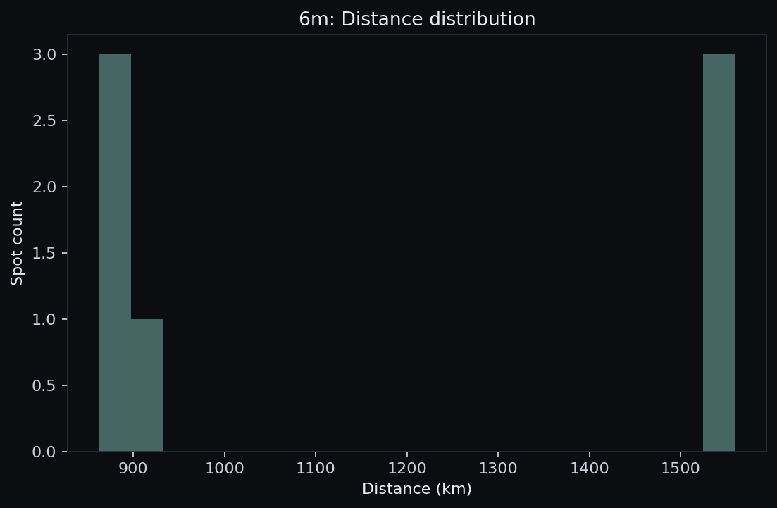
1. Per-band Es/F split. Short-range distance histograms were smoothed and a threshold was selected; values were then clamped to a sensible range. On 6 m a higher threshold was adopted, because paths there were typically Es.
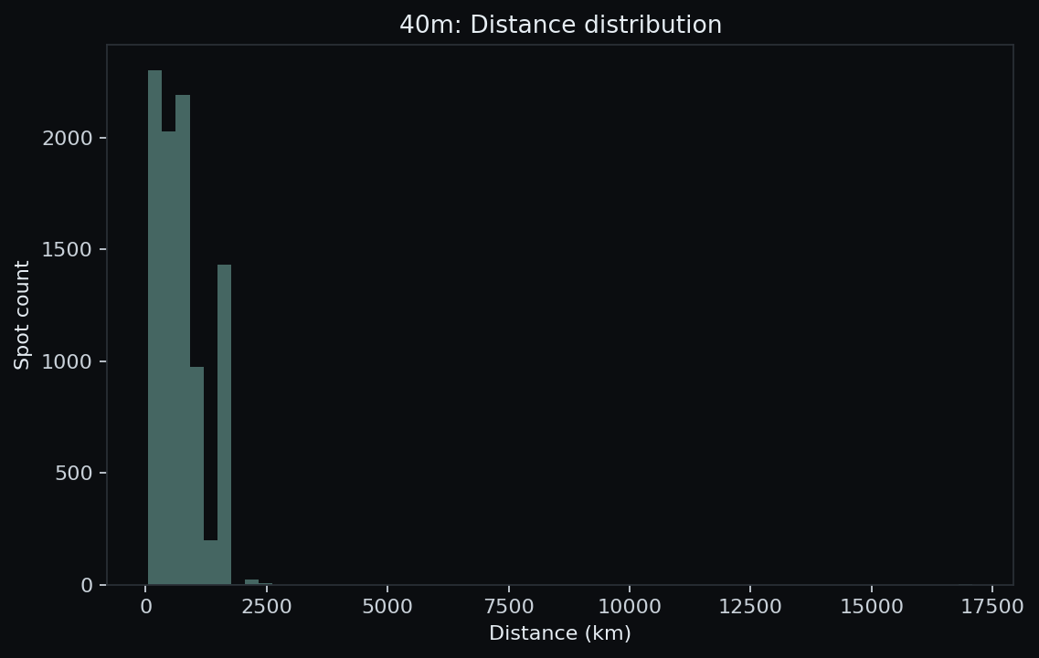
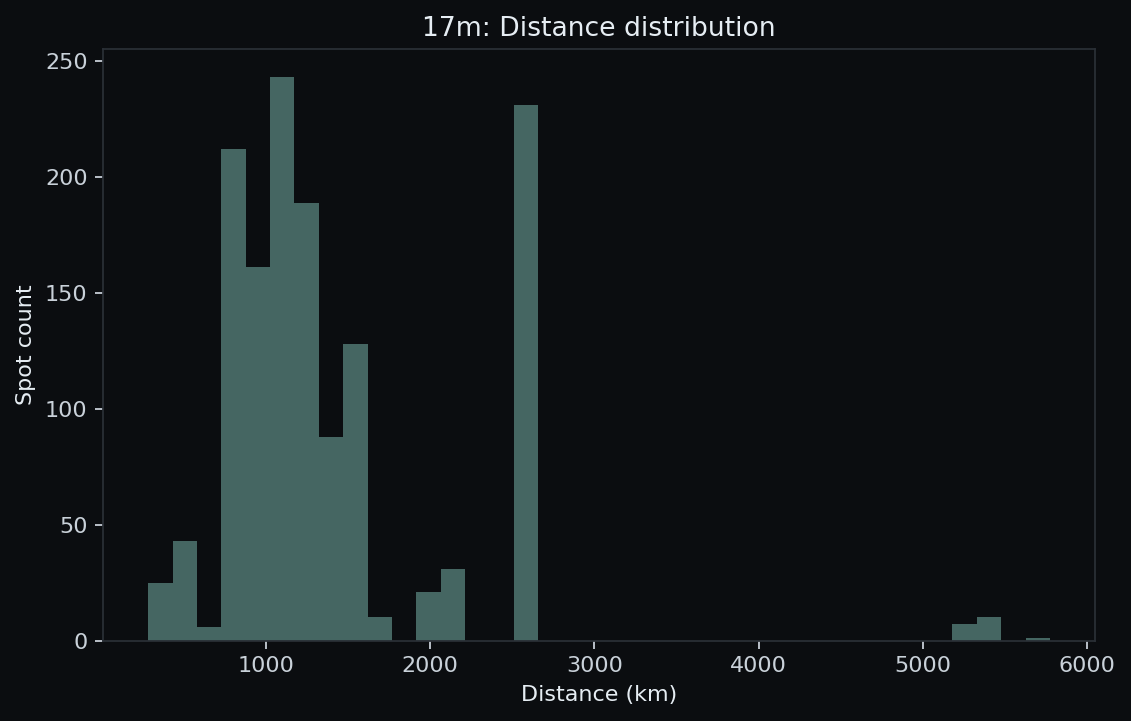
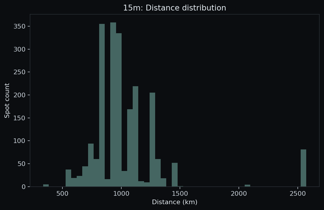
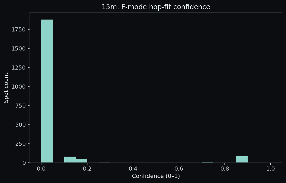
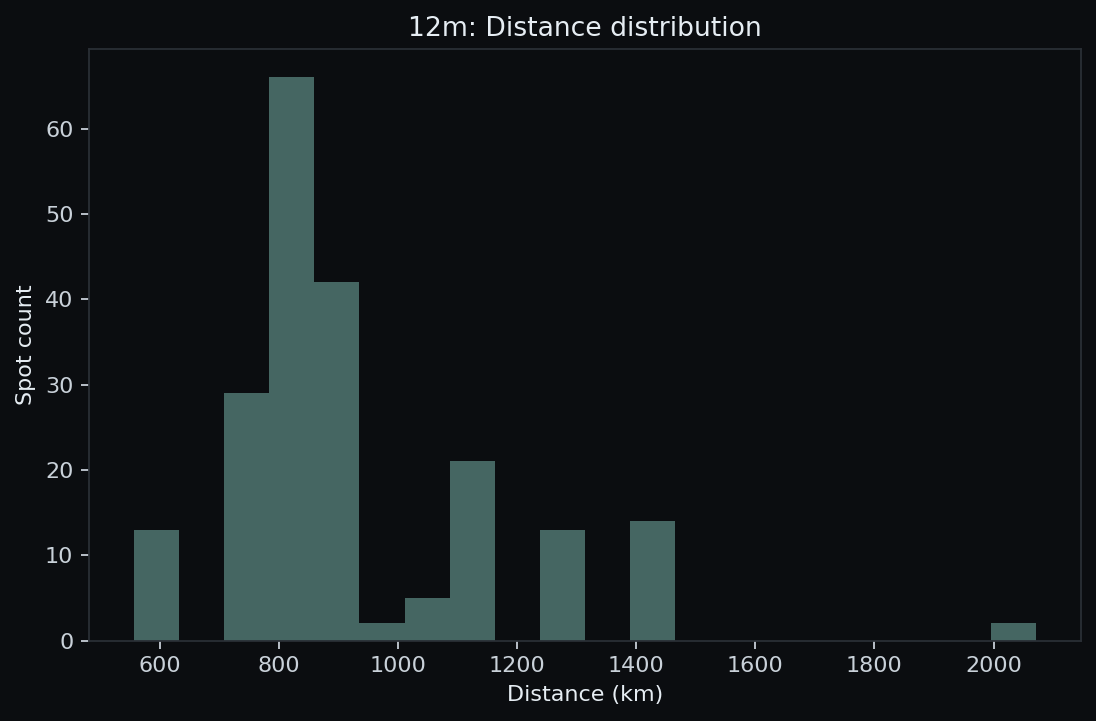
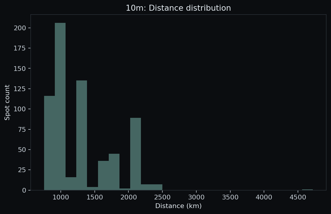
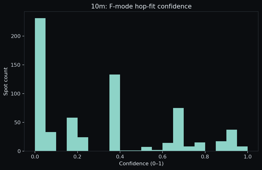
2. F single-hop spacing (μ). The distance histograms exhibited a comb at multiples of an underlying hop length. A seed μ was estimated from that periodicity, refined by minimizing the spread of distance mod μ, and finally tuned by a short grid search per band and for day/night.
3. Heights. Virtual reflection heights of approximately 340 km (F, day), 280 km (F, night), and 110 km (Es) were used.
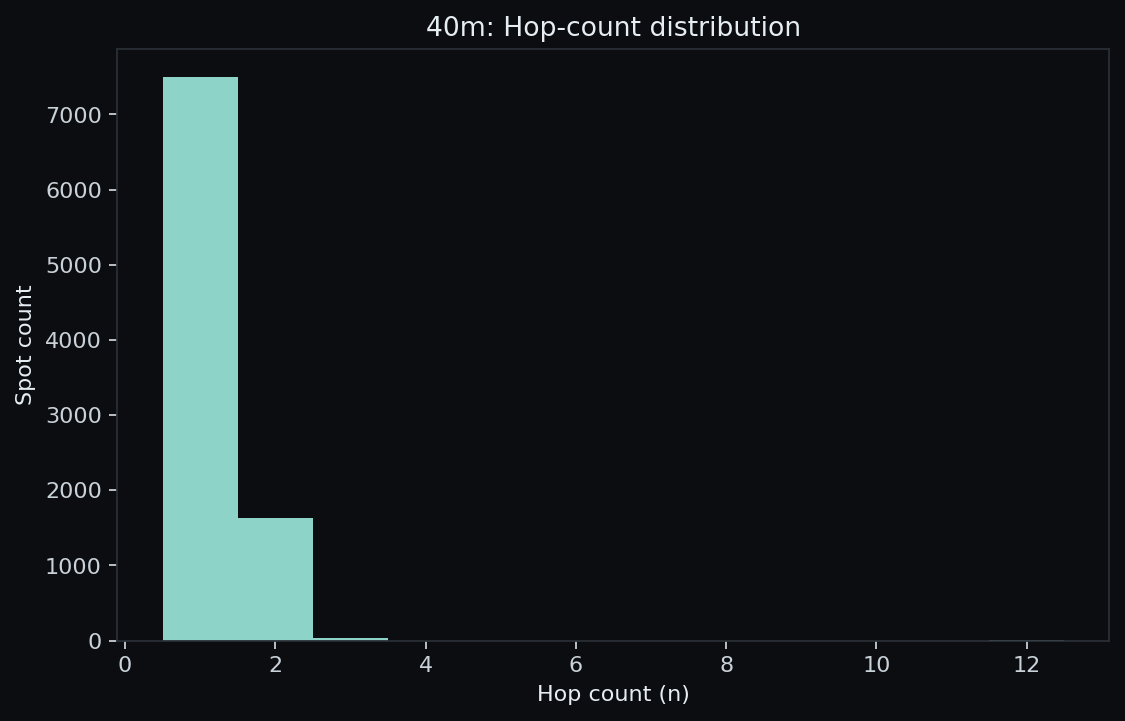
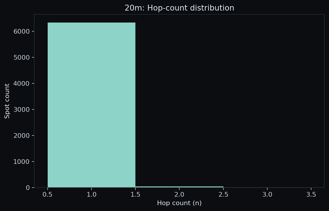
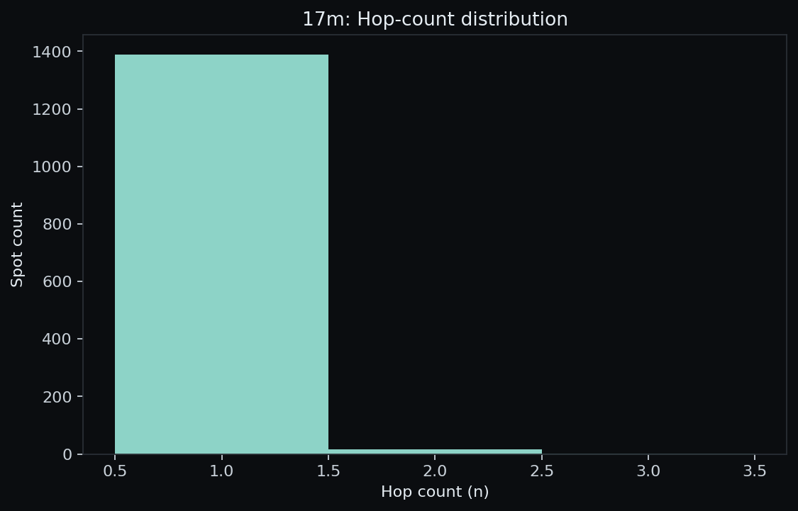
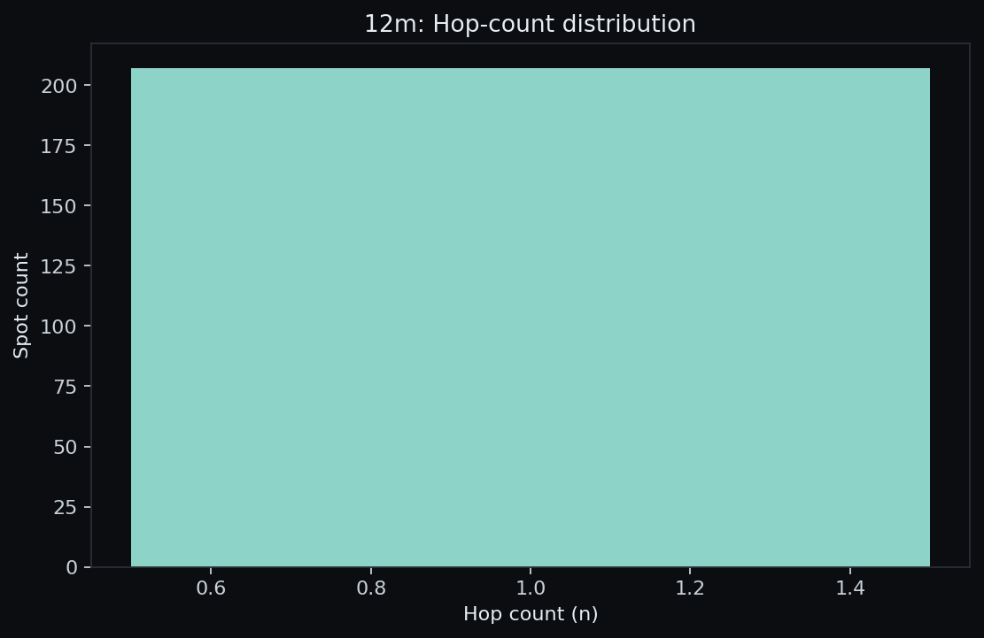
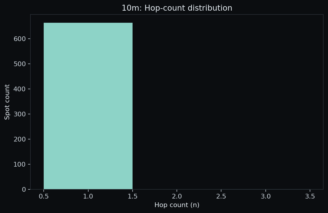
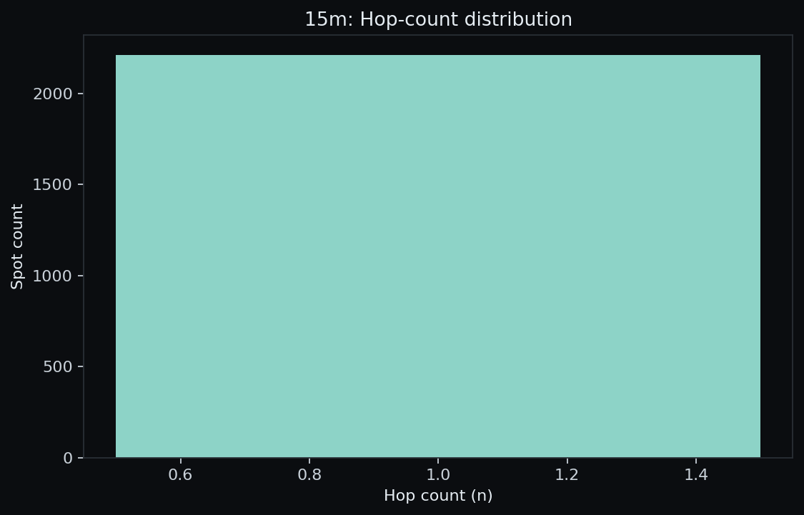
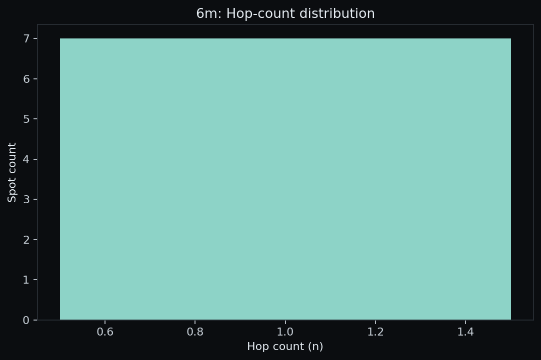
4. Hop count. For F-mode, n ≈ round(D/μ) was used with guards against sub-hop artefacts and unrealistic values. For 6 m, multi-hop Es counts were optionally reported using a nominal Es hop length.
5. Geometry. The take-off angle was the elevation that reached one hop of D/n at the chosen virtual height on a spherical Earth. No path loss modelling was applied—this was geometry only.

This approach was geometry-rigorous but ionosphere-approximate; it was appropriate for interpreting which angles were likely used by the spots actually observed.

Reading the results

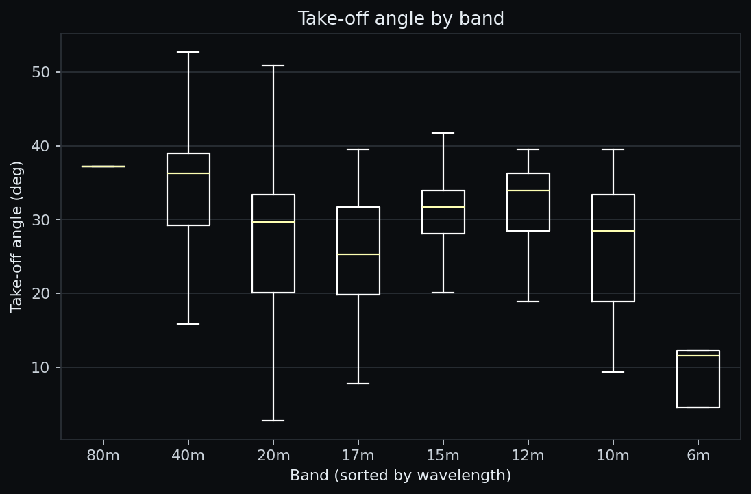
• Typical DX angles. On 20/17/15 m, long paths commonly clustered in the low-angle regime (roughly single-digit to low-teens degrees).
• Why 40 m looked “shorter-hop”. Higher average launch angles (plus daytime D-layer absorption) tended to shorten per-hop ground ranges compared with 20/17/15 m.
• 6 m was Es-dominated. At mid-latitudes, F2 at 50 MHz was rare; multi-hop Es and, seasonally, TEP were more typical drivers of long 6 m paths.

Limits & uncertainty

Single virtual heights, equal hop lengths, and great-circle propagation were assumed; off-great-circle tilts, ducts and full ray-tracing were not modelled. Median take-off angles were expected to carry a small systematic uncertainty (a few degrees), which was acceptable for band-to-band comparisons. Known outliers and implausible distances were capped or excluded to avoid misleading tails.

Where the ionosphere numbers came from

The ionosphere is measured continuously by national and international networks; those measurements informed the typical heights and day/night behaviour used here. Key sources include:

• GIRO / DIDBase (UML-GIRO): Global ionosonde network with ionograms and derived parameters (foE, foF1, foF2, hmF2). Project home · DIDBase (scaled parameters)
• NOAA NCEI: Near real-time and archived ionospheric parameters, plots and station data. Real-time ionosphere · Ionosphere data portal
• International Reference Ionosphere (IRI): Empirical climatology of electron density and F-region parameters used as a reference. IRI model · NASA CCMC IRI
• Spaceborne radio-occultation (e.g., COSMIC-2): Global electron-density profiles derived from GNSS occultations, complementing ionosonde coverage. COSMIC-2 data overview
• Regional examples: Long-running European stations near this QTH. UKSSDC / Chilton (UK) · RMI Dourbes (Belgium)

These external datasets motivated the simple geometric assumptions (e.g., typical F/Es heights). They were not measured by the author of this page.