Hmmm… that’s interesting!

Event summary

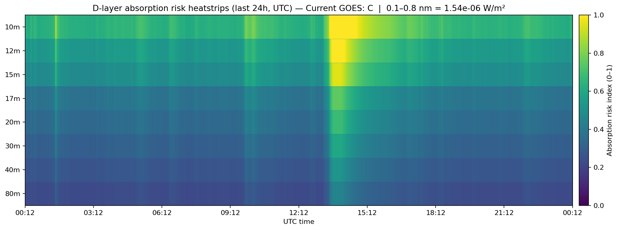
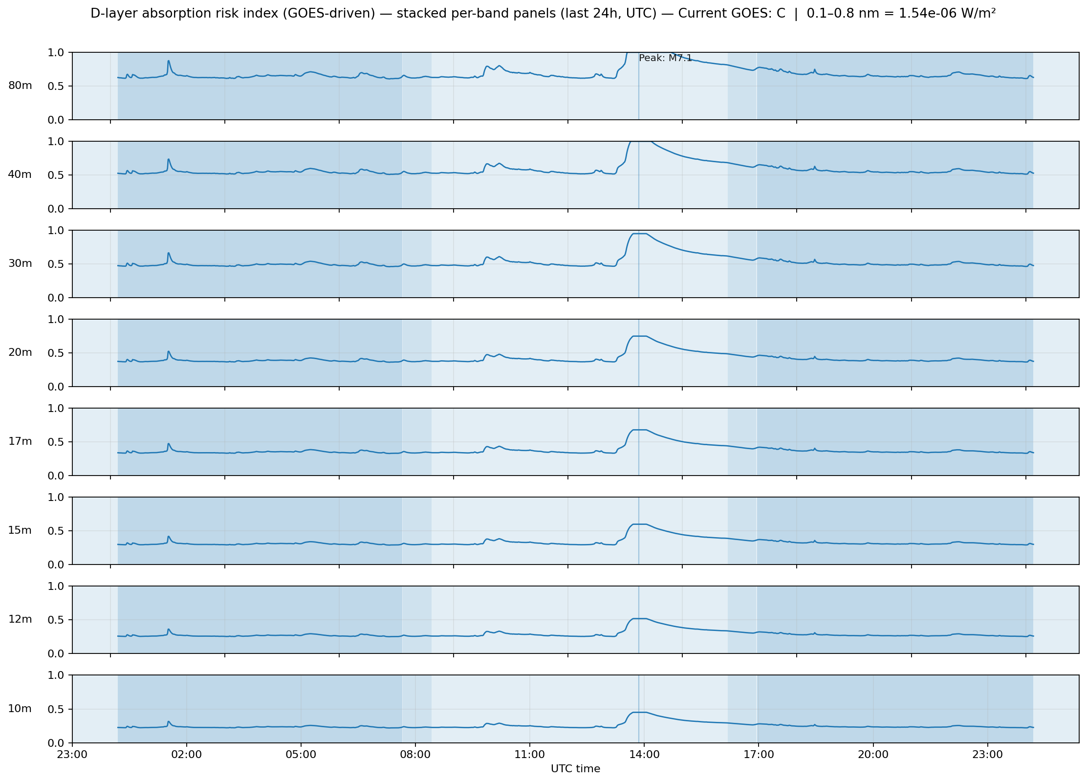
During this event, I noticed a consistent delay between space-weather signatures and local HF propagation effects. When examining multiple independent indicators — space-weather monitors, DRAP/D-layer absorption estimates, and real on-air behaviour — the lag was unmistakable.

The “something just happened” indicators reacted quickly in the data, but the impact on HF propagation in my mid-latitude observation paths occurred later — marked by fewer spots, lower SNR, and a general sigh from the bands.

DRAP / D-Layer plots (last 24 h)

GOES Data:

Heatstrips (24 h):

Stacked view (24 h):

Timing note

Interpretation

The most likely explanation is not an instantaneous global response, but a delayed propagation effect associated with changing ionospheric structure along the relevant path. A flare can increase ionisation rapidly, especially in the lower ionosphere, but the resulting effects on usable HF paths depend on geometry, frequency, and the evolving state of the ionosphere, and therefore do not appear everywhere at once.

One plausible mechanism is the development or passage of travelling ionospheric disturbances (TIDs) or related large-scale ionospheric reorganisation following the solar event. In practical terms, the space-weather instruments reacted first, and the propagation path became visibly worse only later.

• Space-weather instruments show the event first
• Ionospheric structure evolves with delay
• HF propagation effects appear once the disturbed region affects the path

Why this matters

Without side-by-side timing alignment, this sort of lag is easy to miss if you only look at one plot or one index. But when solar monitors, D-layer absorption estimates, and actual on-air behaviour are viewed together, the sequence becomes much clearer.

(There’s a brief background note with references below for those who want to dig into the physics behind this.)

Background (for the curious)

Delayed HF effects following solar events are consistent with established ionospheric propagation theory and observed behaviour in HF monitoring studies. Solar flares can rapidly change ionisation, especially in the lower ionosphere, while larger-scale ionospheric disturbances may then alter HF paths over the minutes that follow. TIDs are a well-known contributor to spatial and temporal HF variability.

• Frissell et al. (2022) — First Observations of Large Scale Traveling Ionospheric Disturbances using HF amateur radio reporting networks
• Heitmann et al. (2018) — Observations and Modeling of Traveling Ionospheric Disturbances and their impact on HF propagation
• Hunsucker, R. D. & Hargreaves, J. K. (2003) — The High-Latitude Ionosphere and its Effects on Radio Propagation
  Publisher preview

Notes

• This is observation-first: it documents a timing pattern and a plausible mechanism.
• The delay strongly suggests path-dependent ionospheric evolution rather than a simple instantaneous response.
• Context: SW UK, operating on 12 m on a transatlantic path — your mileage may vary elsewhere.

Event summary

Several days after a strong solar storm (Jan 20^th 2026), HF propagation appeared to recover in headline indicators: Kp settled, solar wind speed declined, and long-distance paths re-emerged. Despite this, FT8/FT4 operation remained unreliable, with frequent incomplete QSOs and inconsistent decodes.

Signals were present and often strong enough to decode, yet exchanges regularly stalled mid-QSO — suggesting that path existence and path usability had diverged.

Interpretation

Exhibit A — average QSO distance plotted against Kp, GOES X-ray flux, and solar-wind speed — shows a clear pattern:

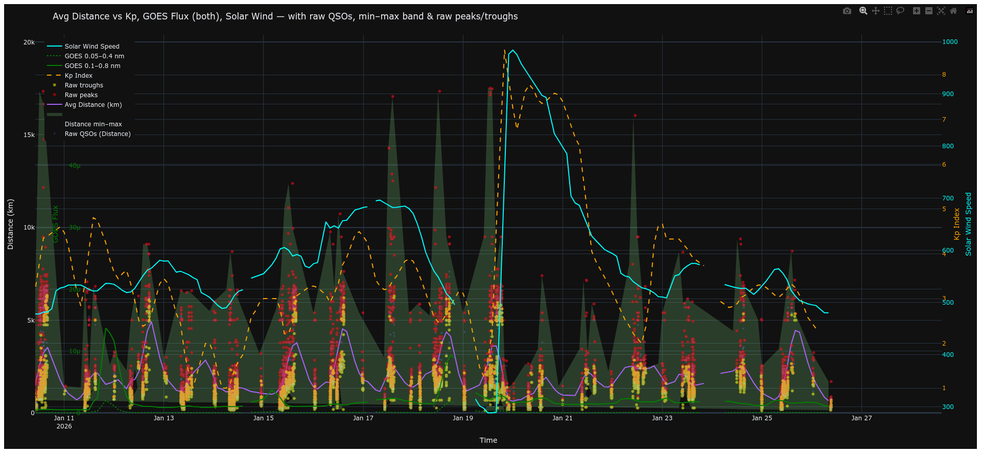
For readers interested in the wider context, the full multi-plot time-series (distance, SNR, Kp, solar wind, GOES flux, band activity, and raw scatter) for this period is available on the Solar Activity & Propagation Dashboard .

Following the solar-wind spike, average distance briefly increases before collapsing and remaining suppressed, even as Kp returns to quiet values. The distance min–max envelope stays unusually wide, indicating unstable refraction rather than simple band closure.

The ionosphere is therefore supporting propagation, but not doing so coherently. Phase stability — critical for FT8 and FT4 — recovers more slowly than distance or signal strength.

What’s likely happening physically

Strong geomagnetic storms do more than temporarily disturb the ionosphere — they can alter its structure for days. Enhanced energy input heats the thermosphere, driving changes in neutral winds and composition that directly affect the F2 layer.

In particular, storm-time circulation can reduce the local O/N₂ ratio at mid-latitudes, lowering peak electron density even after geomagnetic indices have returned to quiet values. The result is an ionosphere that can still refract signals over long distances, but does so inconsistently in time and space.

Superimposed on this are travelling ionospheric disturbances (TIDs) and residual layer tilts, which introduce rapid phase and Doppler variability. These effects are often invisible in headline indices, yet are fatal to phase-sensitive digital modes such as FT8 and FT4.

In short, the F-layer recovers its reach before it recovers its coherence.

In practical terms, the bands are open — but the ionosphere has not yet finished reassembling itself.

Event summary

At the same moment, from the same station, two bands were behaving very differently.

• 20 m → dominated by European stations
• 15 m → dominated by the United States

What was seen

20 m — Europe-dominated activity:

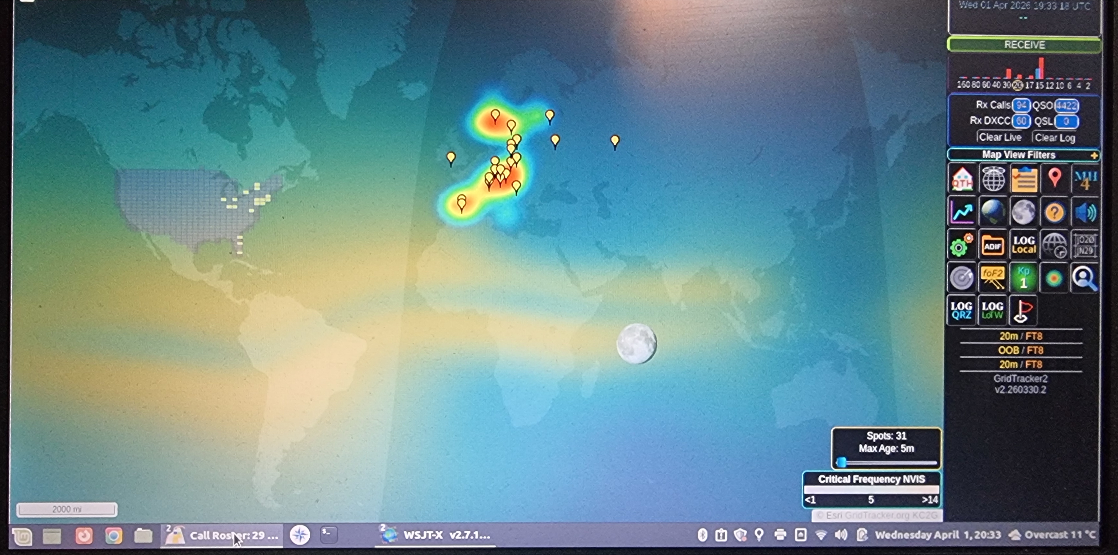
15 m — US-dominated activity:

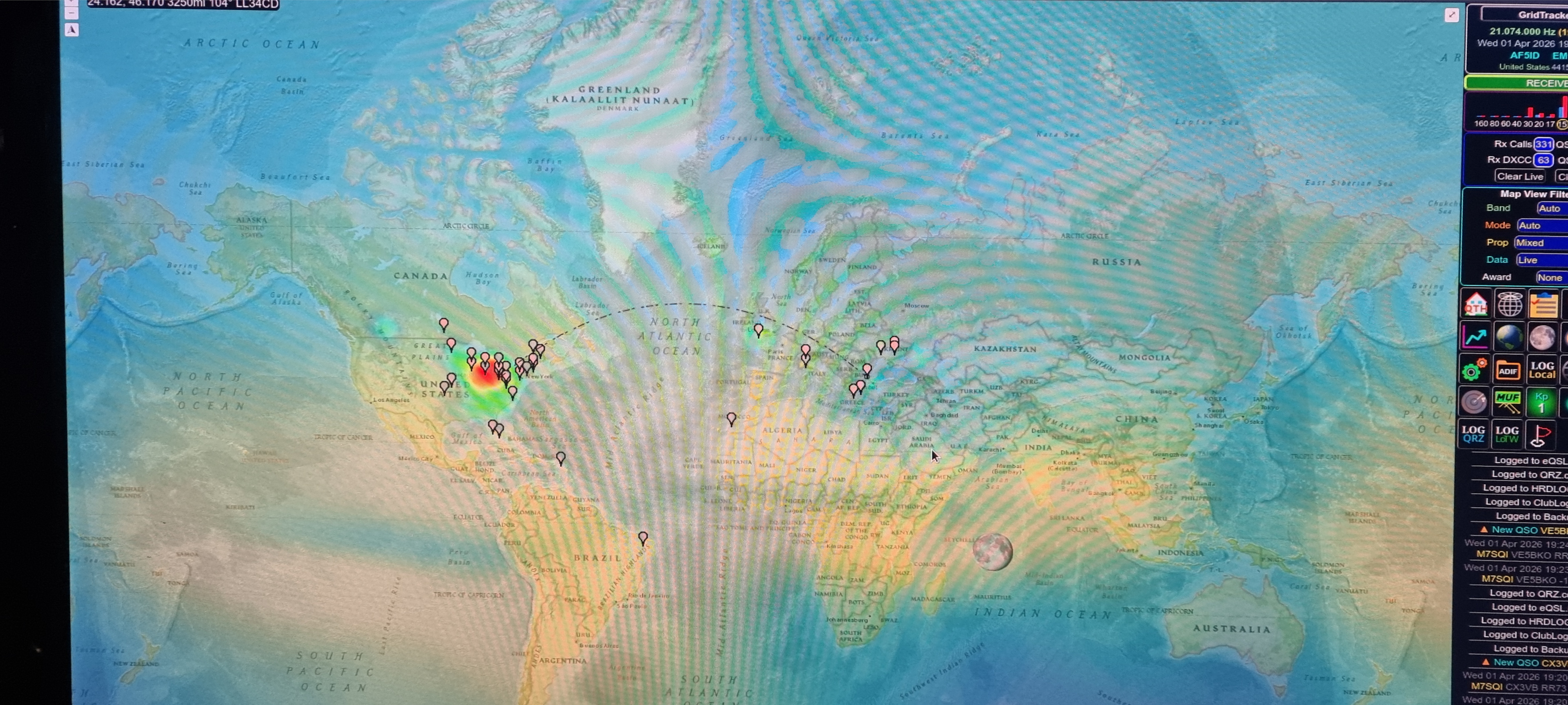
The two maps showed very little overlap, despite being observed at the same time. Each band appeared to be favouring a completely different propagation regime.

Solar context

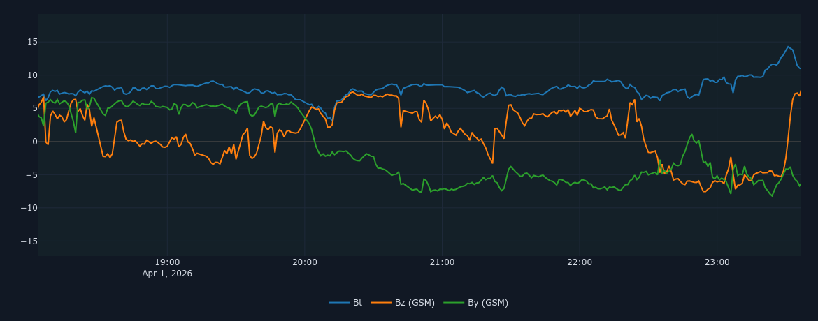
Interplanetary magnetic field (Bt, Bz, By):

GOES X-ray flux (solar activity):

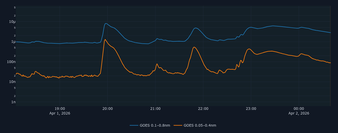
Solar and space-weather conditions showed mild variability, but no significant disturbance that would obviously explain the sharply different behaviour between bands.

• SFI: ~131
• Kp: ~1–2 (quiet)
• Solar wind: moderate (~400–500 km/s)
• Geomagnetic conditions: quiet to mildly unsettled

Interpretation

The most likely explanation is frequency-dependent propagation geometry, driven by differences in takeoff angle and refraction within the F-region.

• 20 m → higher-angle radiation → shorter skip → regional (Europe)
• 15 m → lower-angle radiation → longer skip → transatlantic (US)

This is consistent with the operating frequency of each band relative to the MUF at the time, with 15 m closer to optimum long-path conditions while 20 m favoured shorter, higher-angle returns.

Why this matters

It is tempting to think in simple terms like “conditions are good” or “conditions are poor”. This observation shows that conditions can differ significantly between bands at the same time.

• One band may appear regional
• Another may deliver the DX

(There’s a brief background note with references below for those who want to dig into the physics behind this.)

Practical takeaway

Station note

Observed using a low zig-zag EFHW (~6–20 ft AGL). Dual-rig operation allowed real-time side-by-side comparison.

Background (for the curious)

This behaviour is consistent with established ionospheric propagation theory, in which radio-wave paths depend strongly on frequency, takeoff angle, and electron density structure. Since these parameters vary continuously with time of day and solar illumination, different bands can simultaneously support very different propagation regimes.

Selected references supporting frequency-dependent propagation behaviour:

• Cameron et al. (2022) — HF propagation sensitivity to ionospheric structure
• Cervera et al. — Ionospheric Effects on HF Radio Wave Propagation
• Esmaeili-Karnawah et al. (2024) — Propagation characteristics analysis of HF radio waves in the lower ionosphere
• Davies, K. (1990) — Ionospheric Radio
  ISBN-10: 086341186X
  ISBN-13: 978-0863411861

Final thought

Event summary

A full day of 20 m WSPR data was collected to look for subtle short-term frequency behaviour under mildly unsettled conditions.

(This did, unfortunately, coincide with a day of rather good DX — so instead of working it, I spent the time trying to do “science”.)

The initial result looked dramatic — but for the wrong reason.

Initial view (misleading)

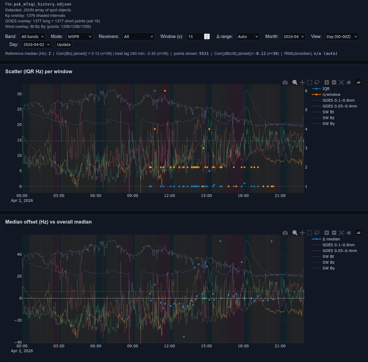
When all tone bins were included, the plot showed large excursions and apparent structure. At first glance, this suggested strong Doppler-like behaviour.

Full dataset (unfiltered view shown above): explore the raw WSPR frequency data

After filtering (what remains)

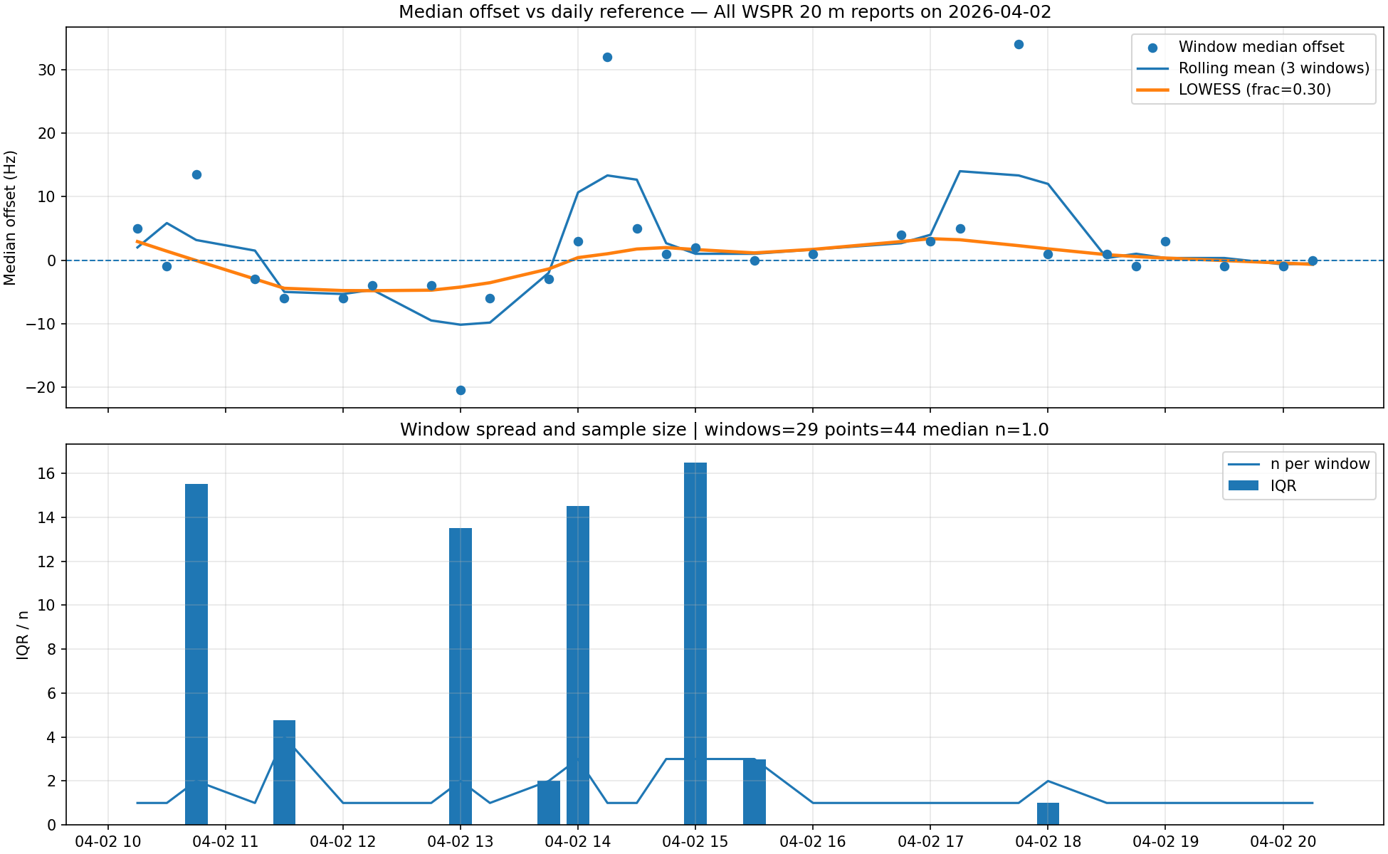
After isolating a single tone cluster, the behaviour changed significantly:

• Large excursions disappeared
• The signal reduced to a few hertz
• A smooth, low-level trend became visible

Method note (what was filtered)

The raw dataset contains reports spanning multiple WSPR tone bins. When combined directly, these appear as large frequency offsets, but primarily reflect tone spacing rather than any physical propagation effect.

To isolate a consistent signal component, the analysis was restricted to a single tone cluster:

• Data filtered to ±50 Hz around the dominant frequency (dataset median)
• This removes mixing between different WSPR audio tones
• Offsets then calculated relative to this filtered reference frequency

This step ensures the plot reflects behaviour within a single transmitted tone cluster. The resulting offsets represent changes in the observed reporting distribution over time, not absolute frequency accuracy or direct Doppler measurement.

🔧 Analysis script: analyze_atmos_wobble_GUI.py

Technical appendix (analysis workflow)

The analysis pipeline follows these steps:

• Load WSPR spot data (JSON input)
• Filter by time window and frequency range
• Determine dominant frequency using dataset median
• Apply ±50 Hz filter to isolate a single tone cluster
• Compute frequency offsets relative to filtered median
• Resample into fixed time windows (e.g. 2 or 15 minutes)
• Calculate median offset per window
• Compute spread (IQR) and sample size
• Apply rolling mean and LOWESS smoothing

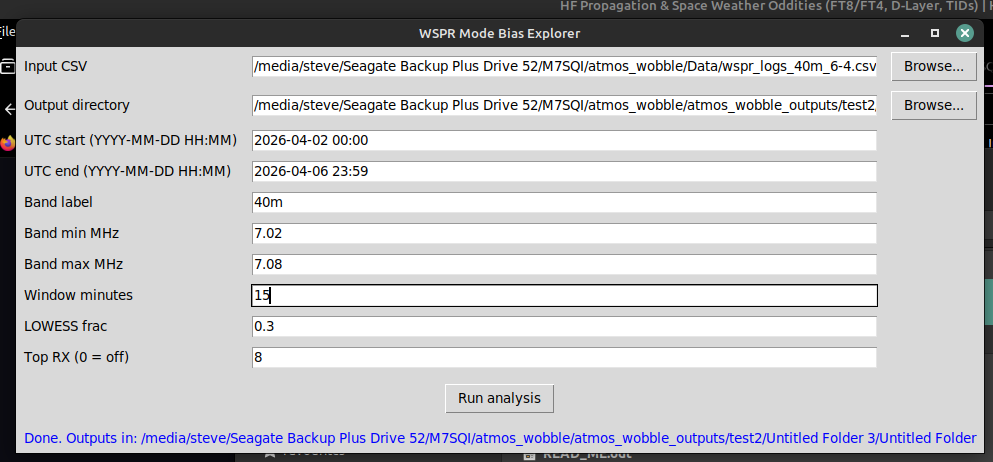
The analysis is controlled via a dedicated analysis interface, allowing consistent selection of time range, frequency bounds, and processing parameters:

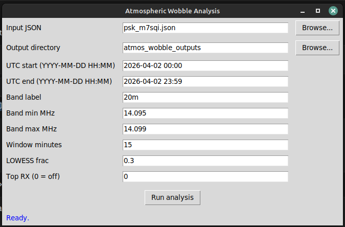
Figure: Analysis interface showing parameter selection for time range, frequency bounds, and smoothing.

The GUI ensures reproducible parameter selection across runs, with all frequency inputs specified in MHz for clarity and internally converted to Hz for processing.

The method is exploratory and intended to highlight structured changes in reporting behaviour, particularly around sunrise/sunset transitions. It is not designed to measure absolute frequency drift or ionospheric Doppler shift.

What was seen

The filtered data shows a gentle diurnal variation:

• slightly negative bias in late morning
• gradual rise through the afternoon
• small positive peak
• return toward zero by evening

The total excursion is only a few hertz, but the trend is smooth and continuous.

Interpretation

This is unlikely to represent a simple Doppler shift in isolation. A more plausible explanation is a gradual change in effective propagation path length, driven by slow evolution of the ionospheric electron density profile — particularly in the F-region.

Small changes in reflection height and electron density can introduce smooth, low-level frequency drift of a few hertz, without requiring rapid motion or strong disturbances. This behaviour is consistent with long-established HF Doppler observations of quiet ionospheric conditions, where gradual changes in effective reflection height produce similar frequency variations over time.

While the effect is small, its smooth and repeatable structure suggests it reflects real ionospheric behaviour rather than measurement noise.

Important caveat

This is not a controlled beacon experiment. The data come from normal WSPR reports, and many time windows contain very few samples.

• Not direct plasma motion measurement
• Not a single-path Doppler experiment
• Interpretation remains cautious

Why this matters

Subtle ionospheric behaviour can hide inside everyday data — but only if the data are cleaned properly first.

Background (for the curious)

Small frequency drifts of this type are consistent with slow variation in ionospheric structure, particularly changes in effective reflection height and propagation path length within the F-region. These effects can introduce smooth, low-level frequency shifts without requiring strong disturbances.

• Davies, K. (1990) — Ionospheric Radio
  ISBN-10: 086341186X
  ISBN-13: 978-0863411861
• Goodman, J. M. (2005) — Space Weather & Telecommunications
  ISBN-10: 0387236708
  ISBN-13: 978-0387236704
  Related publication (DOI)
• Hunsucker, R. D. & Hargreaves, J. K. (2003) — The High-Latitude Ionosphere and its Effects on Radio Propagation
  Preview PDF (Library of Congress)
• Esmaeili-Karnawah et al. (2024) — HF propagation characteristics in the lower ionosphere

Final thought

Event summary

A continuous ~32–34 hour slice of 40 m WSPR data was analysed to investigate whether a small apparent distance-dependent frequency offset structure (ADFOS) might be present.

Equipment: MINI1300 WSPR transmitter (firmware reports 200 mW, actual measured output ≈ 10 mW into 50 Ω).
Antenna: 40 m EFHW at approximately 2 m AGL, site elevation ~100 m AMSL.
Matching: MFJ ATU.
No GPSDO, no external reference, no high-stability modifications — basic setup only.

(This was supposed to be a tidy little follow-up. It turned into a small geography lesson for the ionosphere instead.)

The initial view looked busy and dramatic, but the real structure only became clear after separating the reports by distance.

(If you only look at one result, skip ahead to the distance-band median plot below — that is where the underlying structure becomes clear.)

Live monitoring context

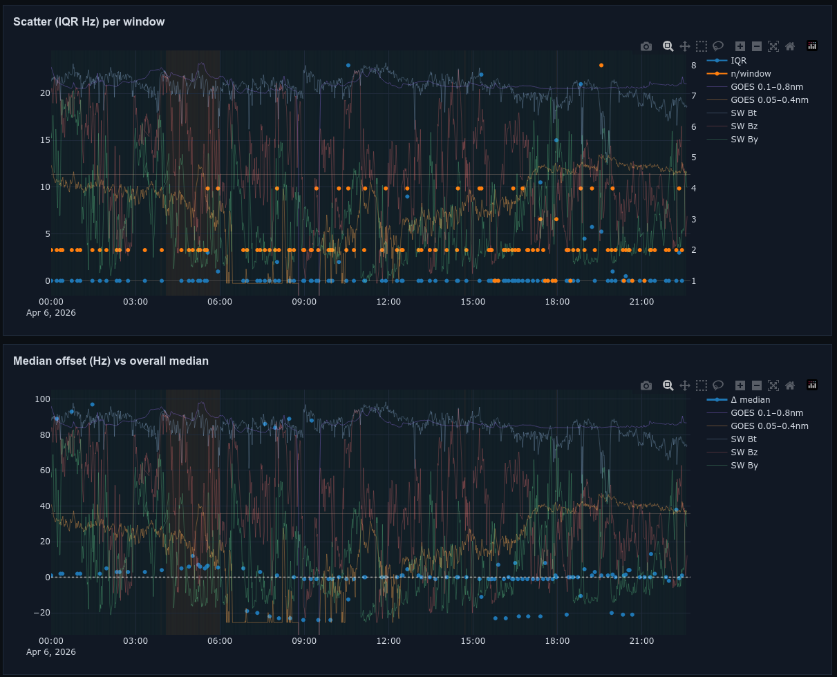
Full dataset (unfiltered view shown above): explore the raw WSPR frequency data

The behaviour was first noticed while monitoring the evolving 40 m dataset alongside space-weather overlays. The live plots were useful for spotting when structure was developing — though not always for understanding what that structure meant.

Mapped WSPR spots (90+ hr window)

👉 Interactive map.

Dense clustering over Europe means many paths share similar azimuths and reflection geometries, limiting true directional separation despite azimuth filtering.

Initial view (misleading)

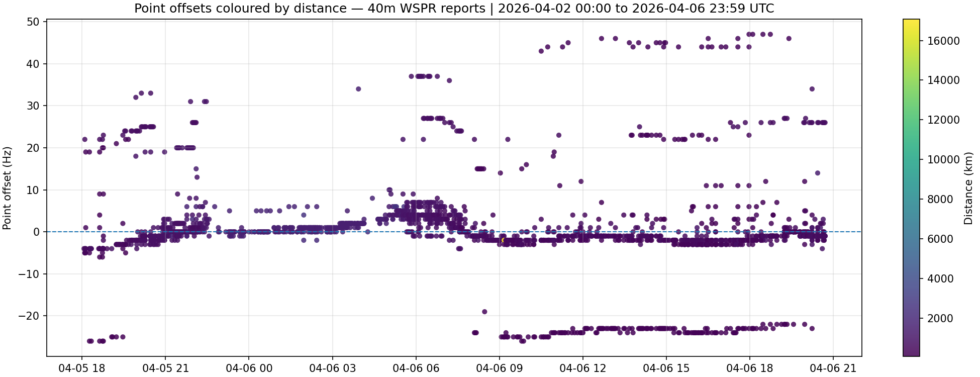
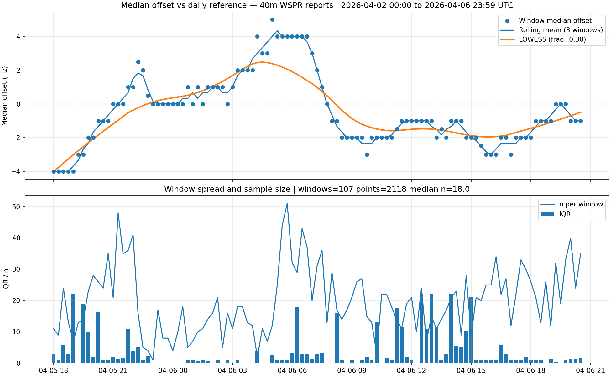
When all reports are viewed together, the plot shows a mixture of strong positive and negative excursions, suggesting a complicated and possibly erratic effect.

In reality, much of this complexity comes from combining very different path lengths into one view.

Full combined-distance view shown above: explore the raw 40 m WSPR frequency data

After separating by distance (what remains)

The figure below is the most important in this section — it shows how each distance band behaves independently over time.

Key figure

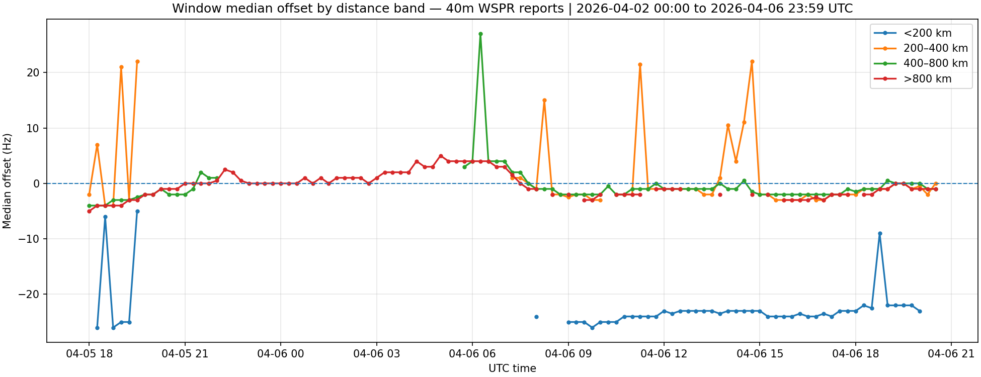
Key result: distance bands evolve differently over time

Once the reports were split into distance bands, the structure became much clearer. This behaviour — referred to here as an apparent distance-dependent frequency offset structure (ADFOS) — is the central observation.

• The <200 km paths formed a persistent negative-offset regime
• The 200–400 km group behaved as a noisier transition region
• The 400–800 km group showed structured positive excursions
• The >800 km paths followed a smoother, lower-amplitude trend

Method note (what was done)

The analysis used the same core approach as the earlier WSPR offset work, but with one extra step: reports were separated into distance bins before comparing their behaviour through time.

To isolate a consistent signal component, the analysis was restricted to a single dominant tone cluster:

• Data filtered to ±50 Hz around the dominant frequency (dataset median)
• Offsets calculated relative to that filtered median reference
• Reports grouped into four path-length bins:
  • <200 km
  • 200–400 km
  • 400–800 km
  • >800 km
• Median offset then examined over time for each group

Offsets are calculated relative to a dataset-derived median reference. This means the zero line reflects the dominant reporting population rather than an absolute frequency standard. The plotted offsets therefore do not represent absolute transmitter accuracy or a direct Doppler measurement. They show how the observed reporting distribution shifts within a single tone cluster — and how that behaviour changes with path length.

Update: per-reporter normalisation removes the global reference bias in the offset scale (which inflated the apparent offsets). View corrected offset plot

🔧 Analysis scripts:
Original method: wspr_mode_bias_explorer_V2.py
Updated (per-reporter normalisation): wspr_mode_bias_explorer_V6.py

Technical appendix (analysis workflow)

The analysis pipeline follows these steps:

• Load WSPR spot data (CSV input)
• Filter by time range and 40 m frequency window
• Determine dominant frequency using dataset median
• Apply ±50 Hz filter to isolate a single tone cluster
• Compute offsets relative to the filtered median
• Assign each report to a distance band
• Plot point offsets by distance and grouped distance band
• Resample into fixed windows and calculate per-band median offset
• Compare repeatability across similar time-of-day slices

The key idea is simple: if all paths behaved the same way, the distance groups would rise and fall together. They do not.

Instead, the shortest paths, intermediate paths, and longer paths appear to form distinct offset regimes, suggesting different propagation geometries are responding differently to the same ionospheric background.

Top-8 reporter subset (supporting check)

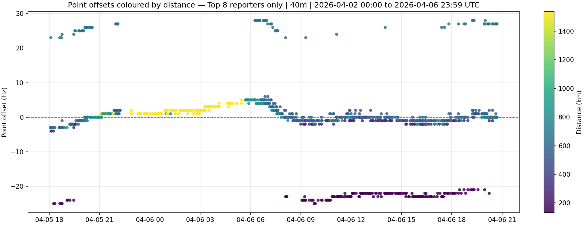
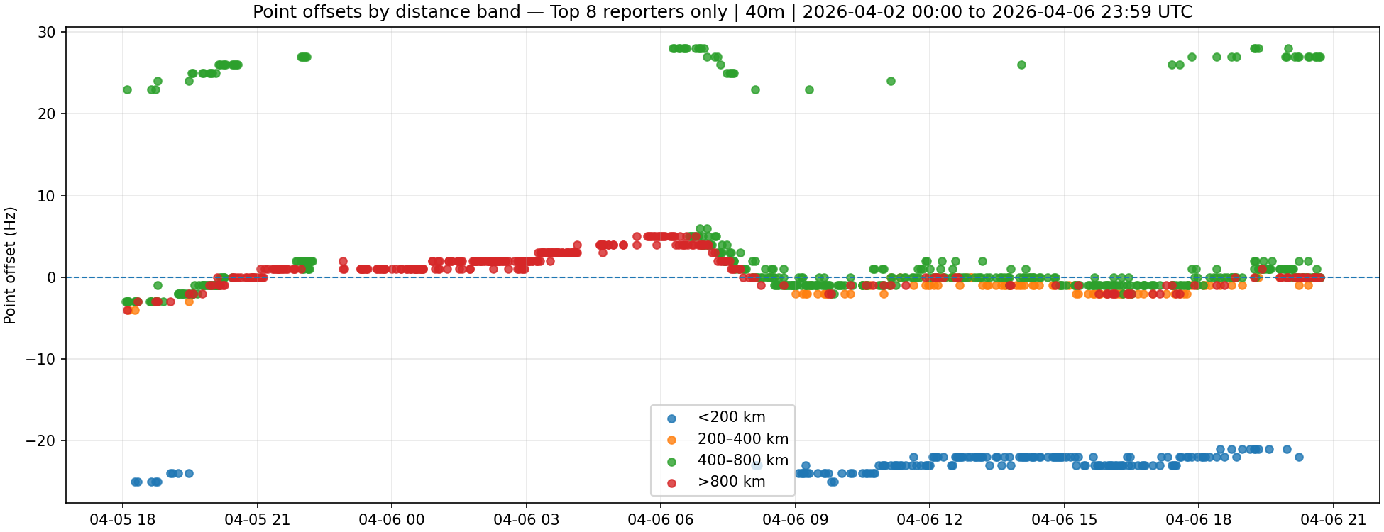
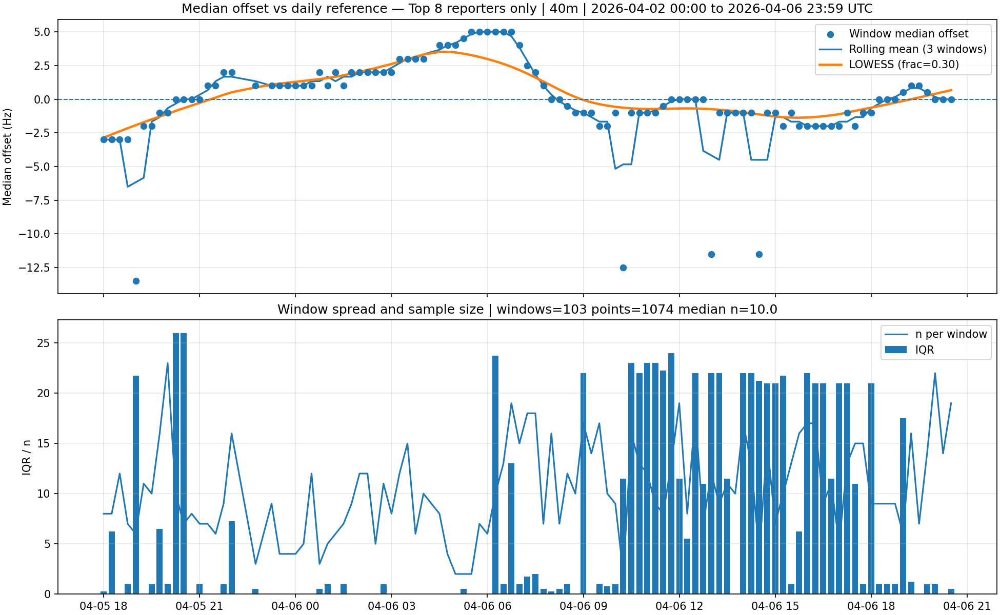
A reduced analysis using only the eight most frequent reporting stations gave a cleaner but broadly consistent picture. The detailed numbers changed, as expected, but the overall separation between path-length regimes remained.

In other words, the pattern does not disappear just because the noisier outskirts of the dataset are trimmed away.

↑ Back to index

Adding solar context: coincidence or clue?

08 Apr 2026 · 40 m WSPR · Extended dataset with solar overlays

Key figure (distance + solar context)

If you only look at one result in this section, make it this one.

Key figure

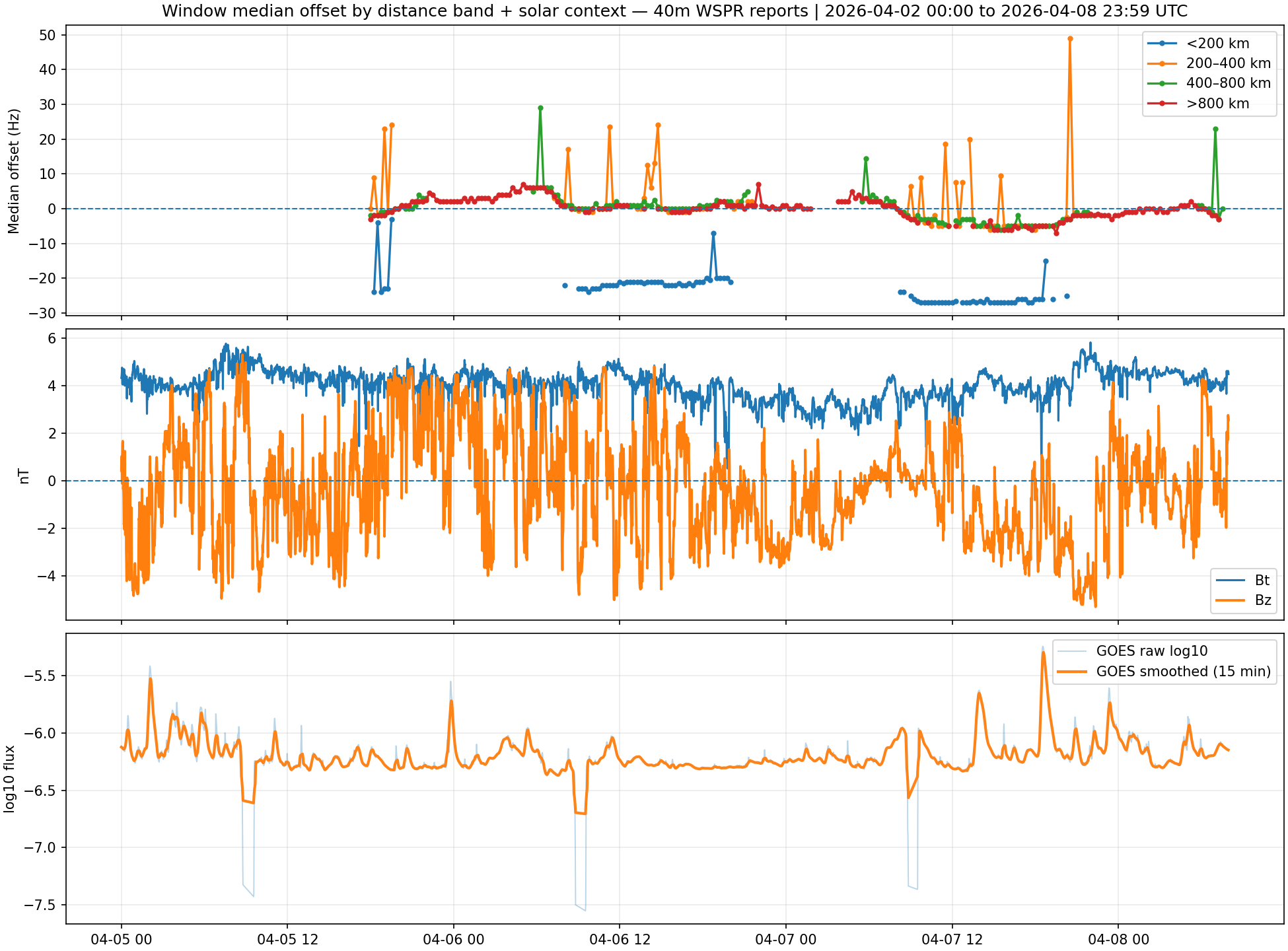
Distance-separated median offset with solar wind and GOES overlays

Top: distance-band median offset
Middle: solar wind (Bt, Bz)
Bottom: GOES X-ray flux (log10, smoothed)

The key feature to watch is how the offset trends evolve relative to the GOES flux variations — particularly during the rising and falling phases of the X-ray signal.

What still holds

Extending the dataset does not weaken the original observation.

• <200 km remains a stable negative-offset regime relative to the reference (~−25 Hz in this dataset)
• 200–400 km remains transitional and noisy
• 400–800 km retains structured positive excursions
• >800 km remains smoother and lower amplitude

The key result — the ADFOS — survives longer duration and additional data.

Geomagnetic context (Bt / Bz)

The solar wind magnetic field shows significant variation, including multiple negative Bz intervals that would normally indicate geomagnetic coupling.

However, there is no consistent alignment between Bt/Bz structure and the observed frequency offset behaviour.

In short: plenty of magnetic activity — but no clear fingerprint in the offset data.

GOES X-ray flux (something… but not clean)

The GOES X-ray flux shows several modest enhancements across the observation period.

Enough to justify plotting it. Not enough to claim causation.

Supporting views

The following plots show the raw structure behind the key result.

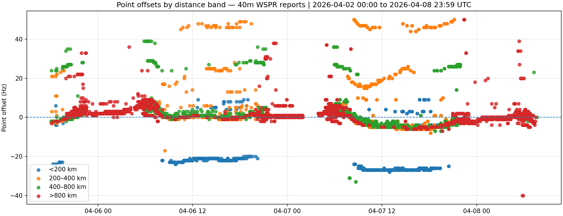
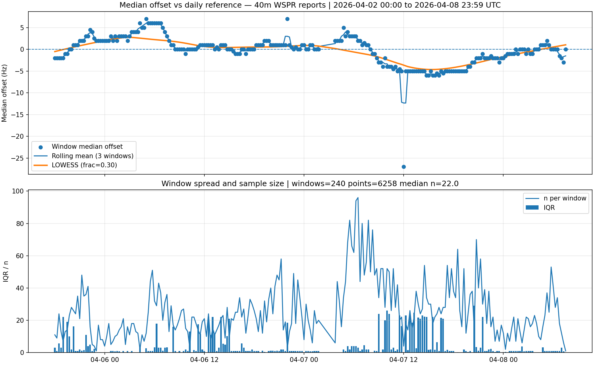
The raw scatter remains complex, but the structured behaviour re-emerges consistently in the windowed median view.

Top-8 reporter subset (sanity check)

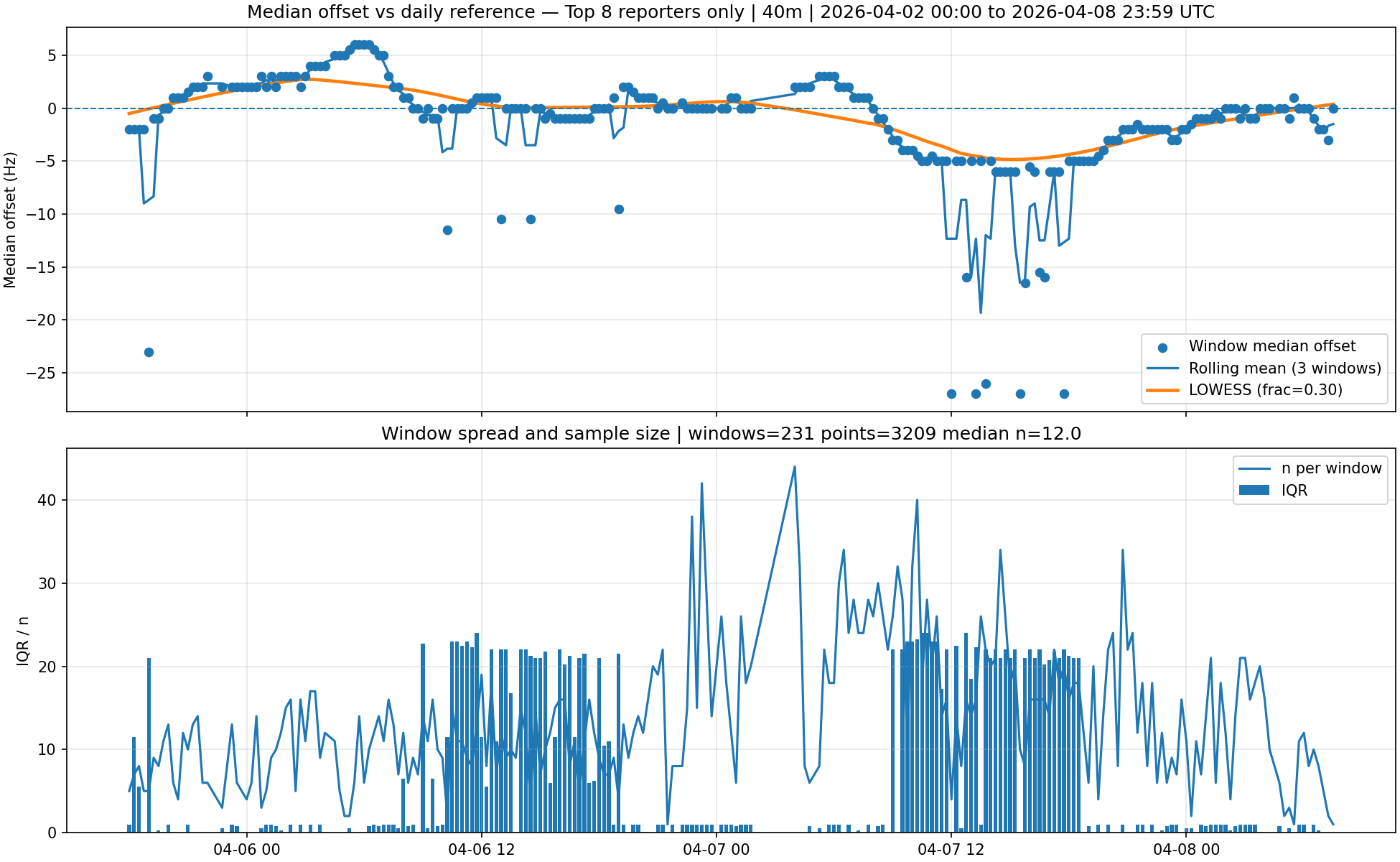
Restricting the dataset to the most active reporters produces a cleaner but consistent version of the same structure.

The effect is not dependent on the long tail of sparse reports.

Method note (extended)

• Same ±50 Hz tone-cluster filtering as Entry 5
• Distance band separation unchanged
• Median offset computed in fixed time windows
• Solar data parsed from HTML source files
• GOES values log-scaled and smoothed (~15 min)

🔧 Updated analysis script: download

(Now with solar data ingestion — because apparently we enjoy making life harder.)

Interpretation

The distance-dependent structure remains the dominant and most reliable result.

Solar context adds a possible secondary influence:

• Geomagnetic field → no clear relationship
• Solar X-ray flux → weak visual correlation

A plausible explanation is that solar-driven changes in ionospheric density subtly alter propagation geometry, affecting path groups differently.

Same ionosphere. Different paths. Different behaviour.

(Or it’s coincidence dressed up as a pattern — which is exactly what the next step needs to test.)

Important caveat

• Not a controlled beacon experiment
• Offsets are relative, not absolute Doppler
• Solar comparison is visual, not statistical

This is a consistent observational pattern — not a confirmed mechanism.

Next step

• Quantify GOES correlation (not eyeballing it like cavemen)
• Test time-lag relationships
• Repeat on other bands

Final thought

The structure survived more data.
The solar link is… suggestive.
The story is not finished yet.

↑ Back to index

Addendum: does receiver mixing hide a lag?

One possible explanation for the weak solar relationship was that the dataset combines reports from many geographically separated receivers. If different locations respond to solar forcing at different times (or even in different directions), any real lagged relationship could be smeared out or cancelled.

To test this, the analysis was repeated using progressively smaller subsets of reporting stations.

Top 4 reporters

Reducing the dataset begins to clarify the distance-dependent structure, but the solar context remains difficult to interpret.

Top 2 reporters

With fewer receivers, the WSPR offset behaviour becomes smoother and more coherent. However, no consistent alignment with solar parameters is revealed.

Single reporter (near single-path geometry)

Isolation test

Geometry simplified to a single receiver — no consistent solar-linked lag observed

When reduced to a single reporting station, the offset trace becomes a clear, continuous temporal structure. This effectively removes spatial averaging effects from the dataset.

If a consistent solar-driven lag were present, this is where it should become visible.

No such relationship emerges.

Result

Across all levels of receiver reduction:

• The ADFOS remains robust
• The WSPR signal becomes progressively clearer
• No consistent temporal alignment appears with Bt, Bz, or GOES X-ray flux

Occasional visual similarities occur, but they are not repeatable or stable enough to support a causal relationship.

Interpretation

This test removes one of the main sources of ambiguity — spatial averaging — yet the expected lagged relationship still does not emerge.

This suggests that:

• The lack of correlation is not caused by receiver mixing
• If a solar-driven effect exists, it is weak, indirect, or highly localised
• The dominant behaviour remains propagation geometry

Simplifying the geometry clarifies the signal — but does not reveal a hidden solar driver.

Takeaway

Even when reduced to a near single-path observation, the offset structure appears largely independent of the solar parameters examined here.

That does not rule out solar influence — but it significantly raises the bar for demonstrating it with this type of data, and points toward the need for direct ionospheric measurements.

In plain terms

The ADFOS is real and repeatable.
It depends strongly on path geometry.
It does not show a consistent relationship with the solar parameters tested here.

Next steps

Why this update was needed

The previous entries

• 06 Apr 2026 — 40m - Apparent distance-dependent offset structure (ADFOS)?
• 08 Apr 2026 — 40m - Adding solar context: coincidence or clue?

documented the investigation as it unfolded: first the identification of a distance-dependent frequency offset structure (ADFOS), and then an attempt to test whether that behaviour might relate to solar or geomagnetic conditions.

Those initial results raised two important questions:

• Was the observed offset scale influenced by the choice of reference?
• Was there a genuine solar-driven component, or only a visual coincidence?

To address this, the analysis was repeated with improved normalisation, extended data, and more controlled testing of lag and receiver-mixing effects.

What changed in the method

The core analysis approach remains the same as in the earlier entries, but three methodological changes were introduced to remove known sources of bias and improve consistency.

• Per-reporter normalisation
  Offsets are now calculated relative to each reporter’s local reference, rather than a single global median. This removes population bias that previously inflated the apparent offset scale.
• Consistent filtering and windowing
  A fixed ±50 Hz tone-cluster filter and standardised time-window smoothing were applied across all runs. Earlier exploratory variations in parameters were removed to ensure comparability.
• Extended dataset
  The analysis window was expanded to ~90+ hours, allowing behaviour to be examined across multiple diurnal cycles rather than a single slice.

What survived correction

Repeating the analysis with per-reporter normalisation significantly reduces the apparent offset magnitude seen in the earlier plots. However, the key observation remains unchanged.

Key figure

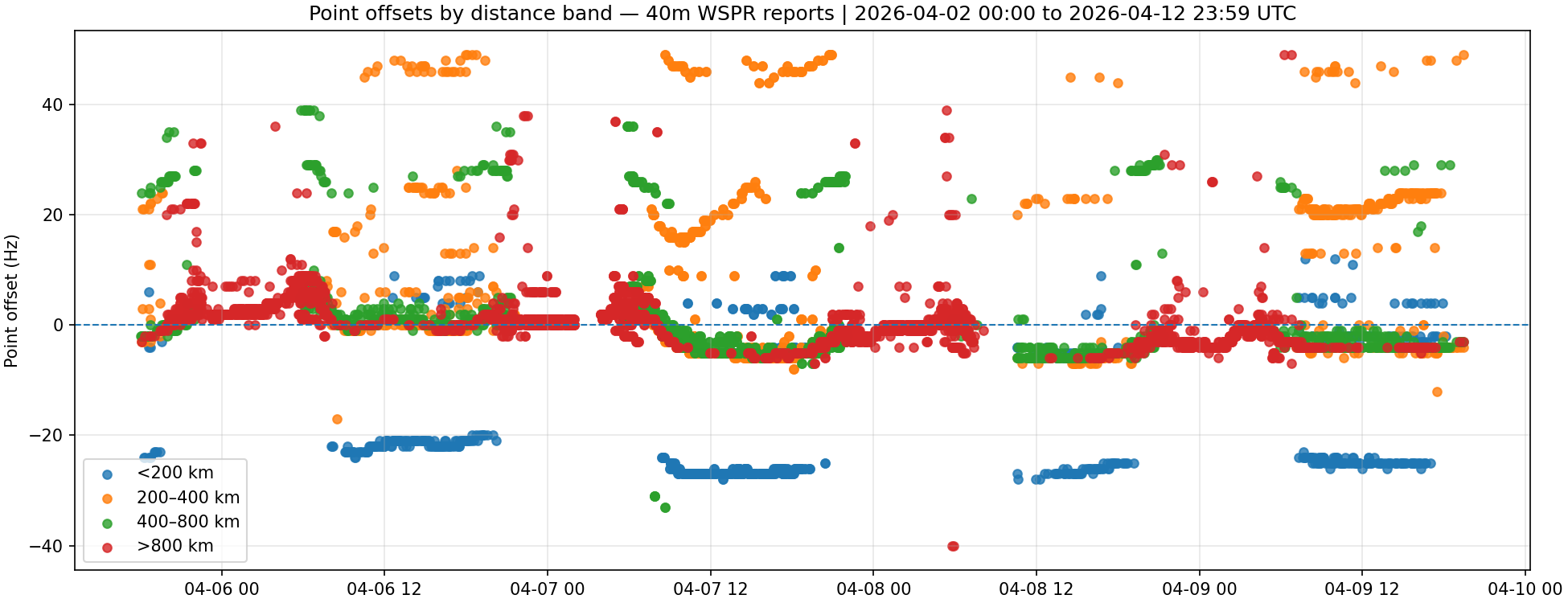
A single global median introduced a population bias that inflated the apparent offset scale

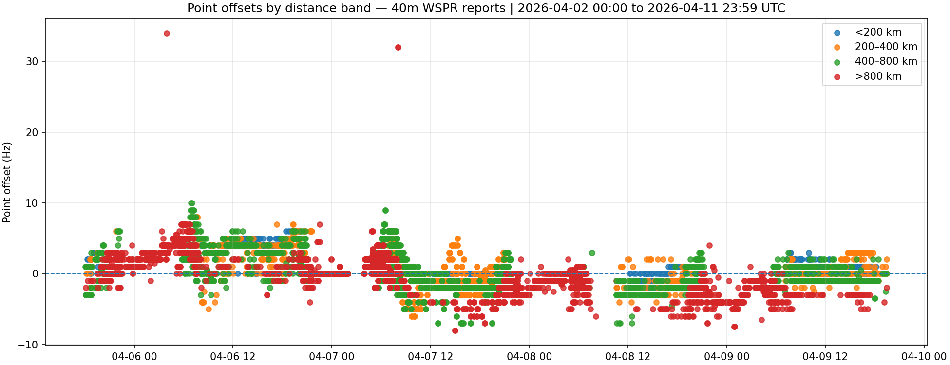
Per-reporter normalisation reduces the offset magnitude while preserving the distance-dependent structure

The distance-separated structure persists: the different path-length groups continue to evolve independently over time, rather than following a single shared trend.

All results shown here are restricted to a single ±50 Hz tone cluster to avoid mixing multiple signal populations. The observed behaviour therefore reflects propagation differences rather than multiple signal populations.

• The distance-separated structure persists, with the different path-length groups continuing to evolve independently over time.
• The shortest-path group is often displaced relative to the longer-path groups, though the degree of separation varies with time.
• Intermediate distance bands show mixed behaviour, often bridging the shorter- and longer-path regimes.
• The longest-path group follows a distinct trajectory of its own, including substantial excursions that do not simply mirror the shorter paths.

The correction therefore changes the scale of the effect, but not its existence.

How the analysis evolved

To understand the results that follow, it is useful to outline how the analysis itself developed.

The analysis did not begin in its final form. Early versions focused on simple global statistics and visual inspection, which were sufficient to identify the initial structure but also introduced several sources of bias.

As new questions emerged, the tooling was extended in stages:

• Initial exploration: global median-based analysis to identify overall offset behaviour
• Distance separation: grouping by path length revealed the structure as distinct populations rather than a single trend
• Per-reporter normalisation: removed population bias and corrected the apparent scale of the effect
• Lag analysis tools: introduced cross-correlation testing to search for delayed relationships
• Sector and azimuth probes: explored whether directional filtering revealed hidden solar coupling
• Receiver reduction: tested whether spatial averaging was masking a cleaner signal

Each step was driven by a specific question raised by the previous results, and many of the later tools were designed specifically to try to break the earlier interpretations.

The later script versions were not replacements so much as extensions: each was added to test a new hypothesis raised by the previous round of results.

🔧 Analysis tools developed during this investigation:
Core analysis (per-reporter normalisation): wspr_mode_bias_explorer_V6.py
Solar comparison + lag testing: wspr_mode_bias_explorer_V7.py
Additional directional/sector tests: wspr_azimuth_lag_probe_V2a.py
wspr_solar_sector_probe_V1.py

What did not survive

Several early interpretations looked suggestive at first glance, but did not remain stable under tighter controls.

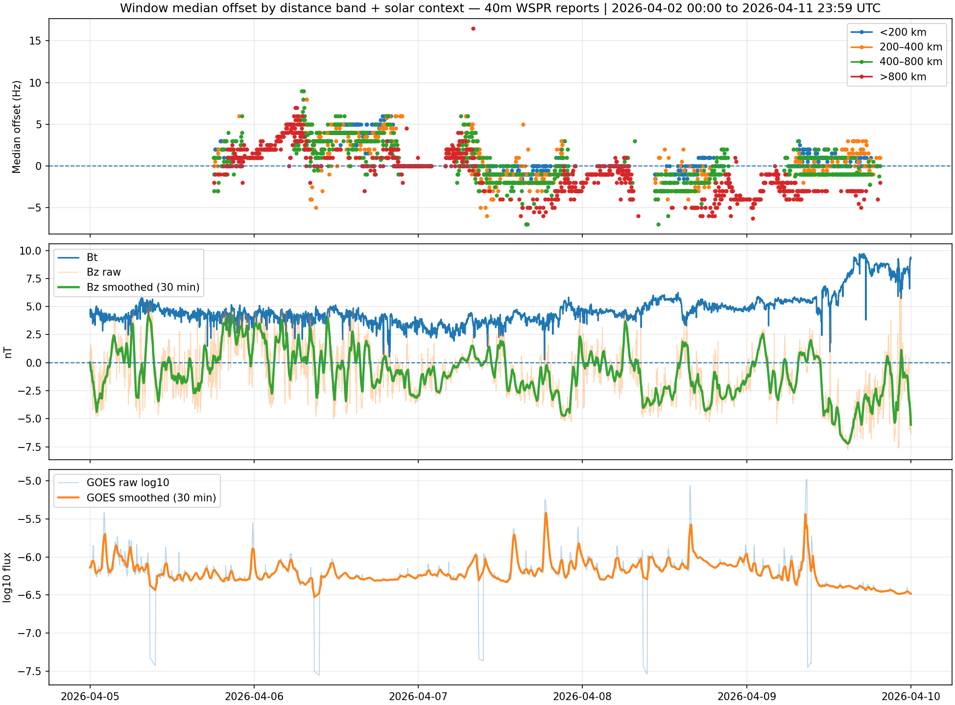
1. A single solar driver

No consistent alignment was found between the offset structure and solar wind magnetic field parameters (Bt, Bz) or GOES X-ray flux. Occasional visual similarities occur, but they are not repeatable or stable enough to support a causal relationship.

Distance-band behaviour compared against solar context over the full dataset

2. A fixed lag relationship

To test whether the observed behaviour could be explained by a delayed response to an external driver, cross-correlation analysis was applied between different subsets of the WSPR data (e.g. azimuth sectors and distance bands). The aim was to identify a consistent time lag that might indicate a causal relationship.

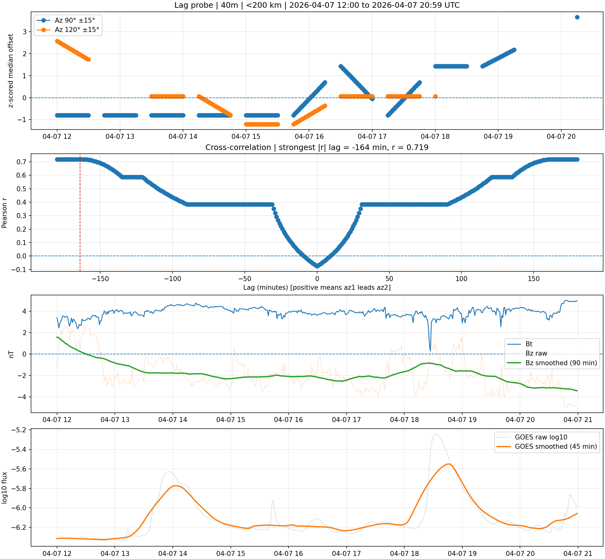
Example of apparent lag behaviour between azimuth sectors. Although cross-correlation suggests a strong lag (~−160 min), the smooth, symmetric correlation structure and lack of consistent alignment in the underlying series indicate trend matching rather than a physical delay.

Even in cases where cross-correlation produced a strong and well-defined lag, the underlying structure did not support a causal interpretation.

Comparison views: Different parameters

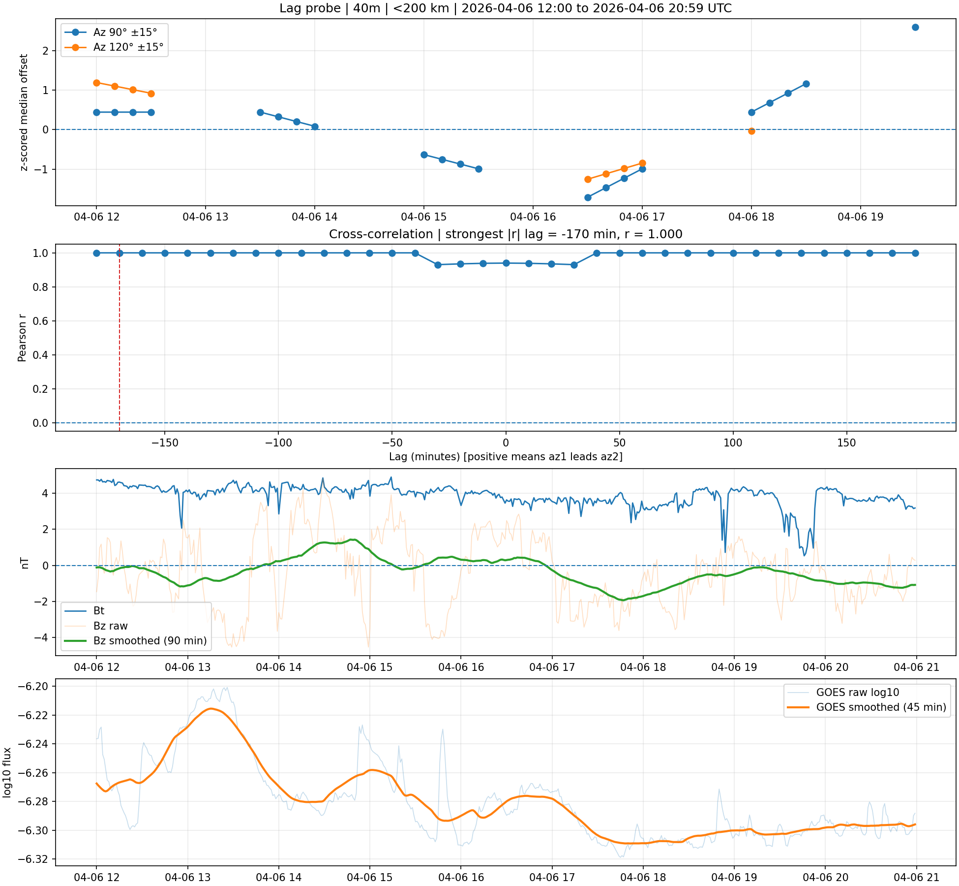
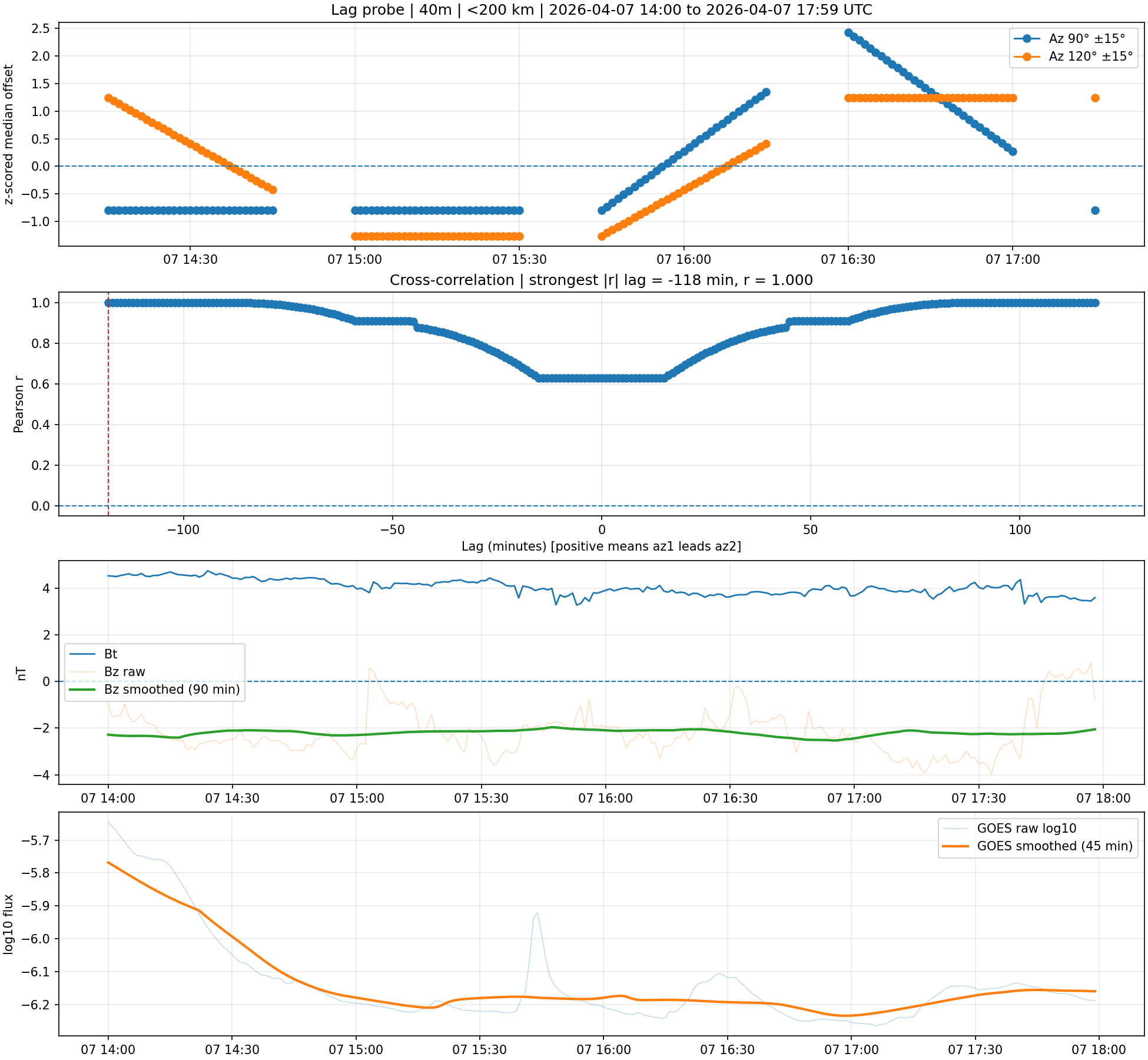
Cross-correlation and lag testing produced broad, unstable, or boundary-hugging peaks rather than a well-defined delay. Similar lag structures appeared across unrelated inputs, indicating trend alignment rather than a physical response time.

3. Directional or sector-based solar coupling

A second approach tested whether any apparent solar relationship might be hidden within specific propagation directions. The dataset was divided into azimuth sectors and distance bands, and each subset was compared against solar and geomagnetic parameters (GOES X-ray flux, Bt, Bz) across a range of lags.

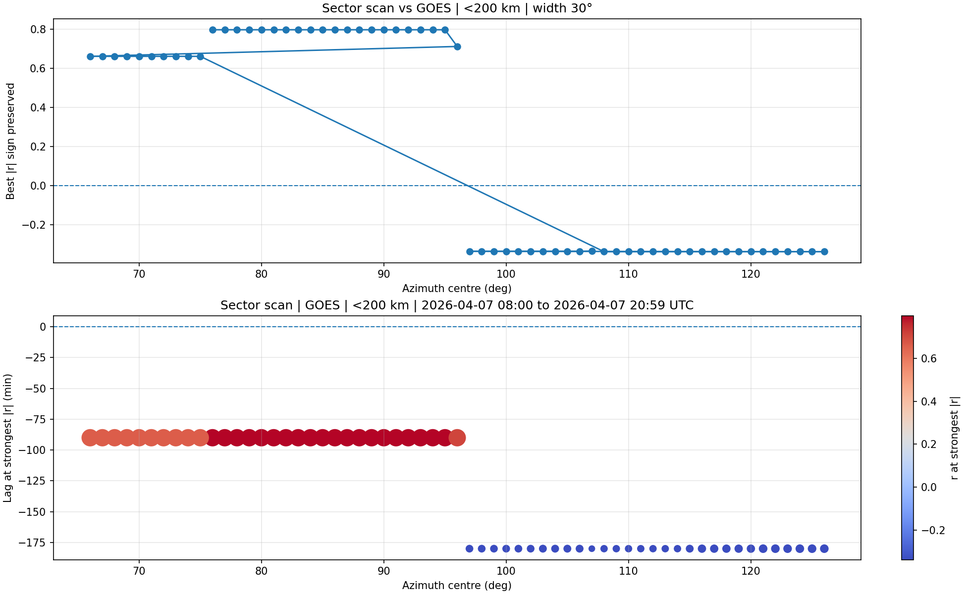
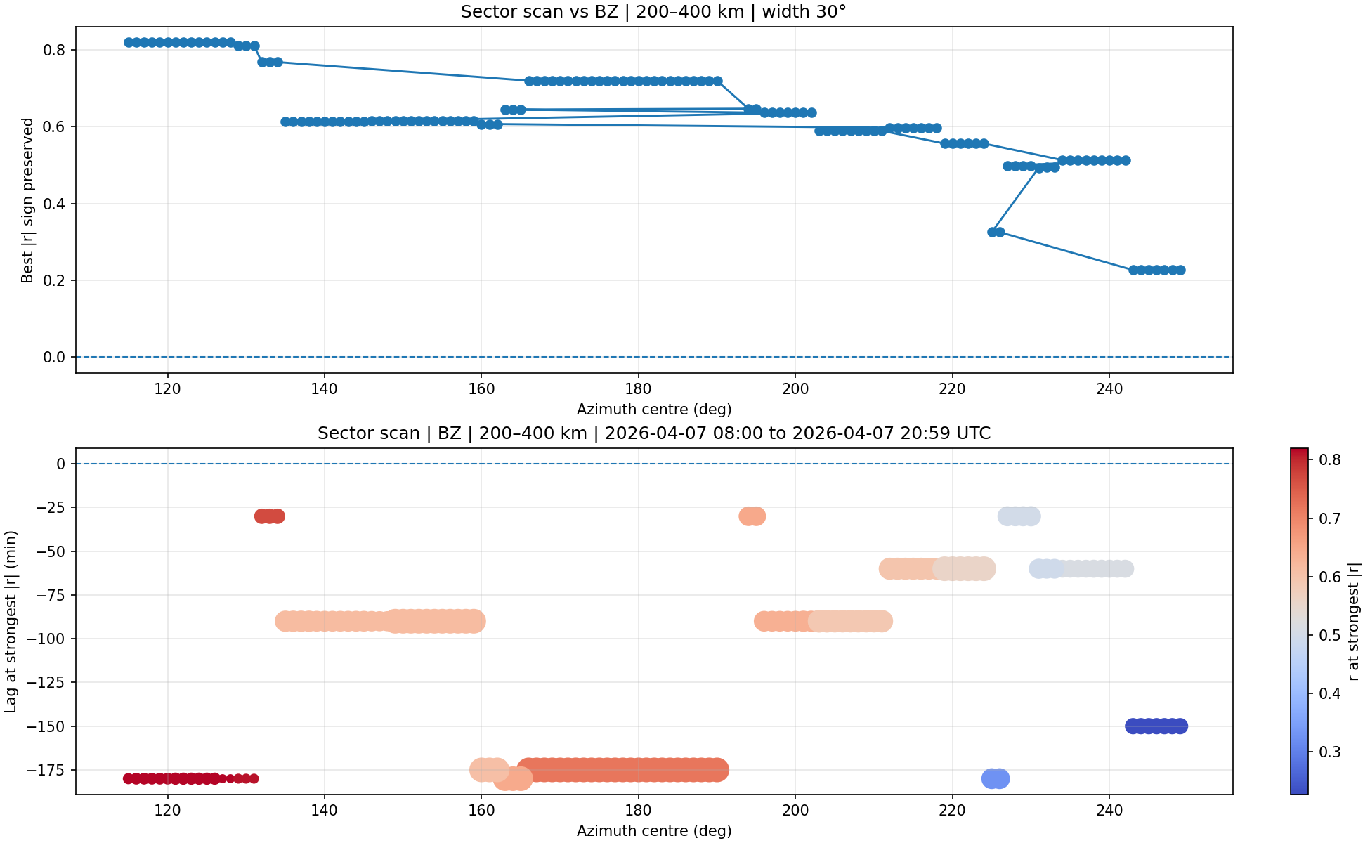
While some sectors produced moderate correlations, these were not consistent in sign, lag, azimuth, or solar parameter. Different combinations gave different answers, which is not what a stable external driver should produce.

Additional directional and sector probe examples

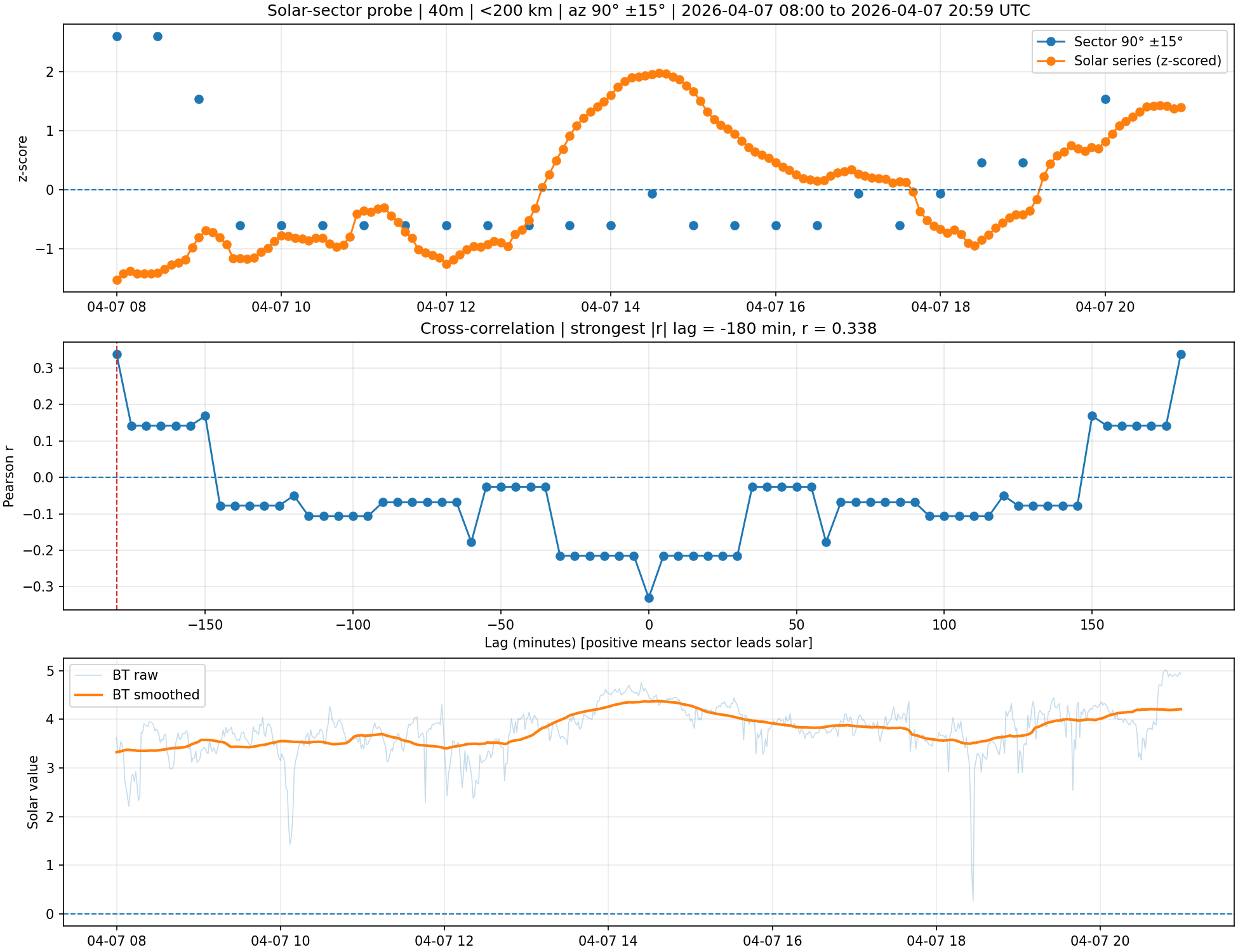
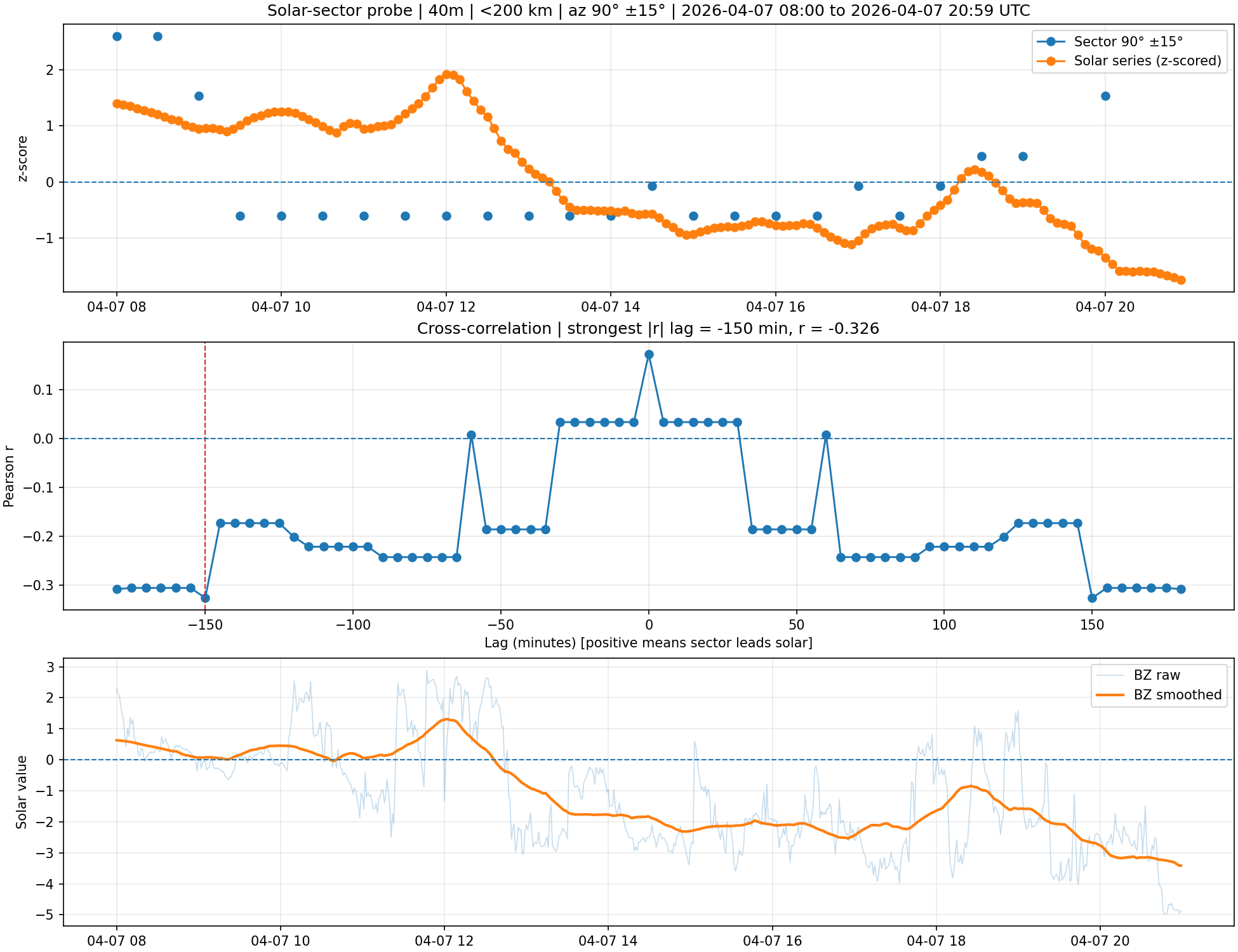
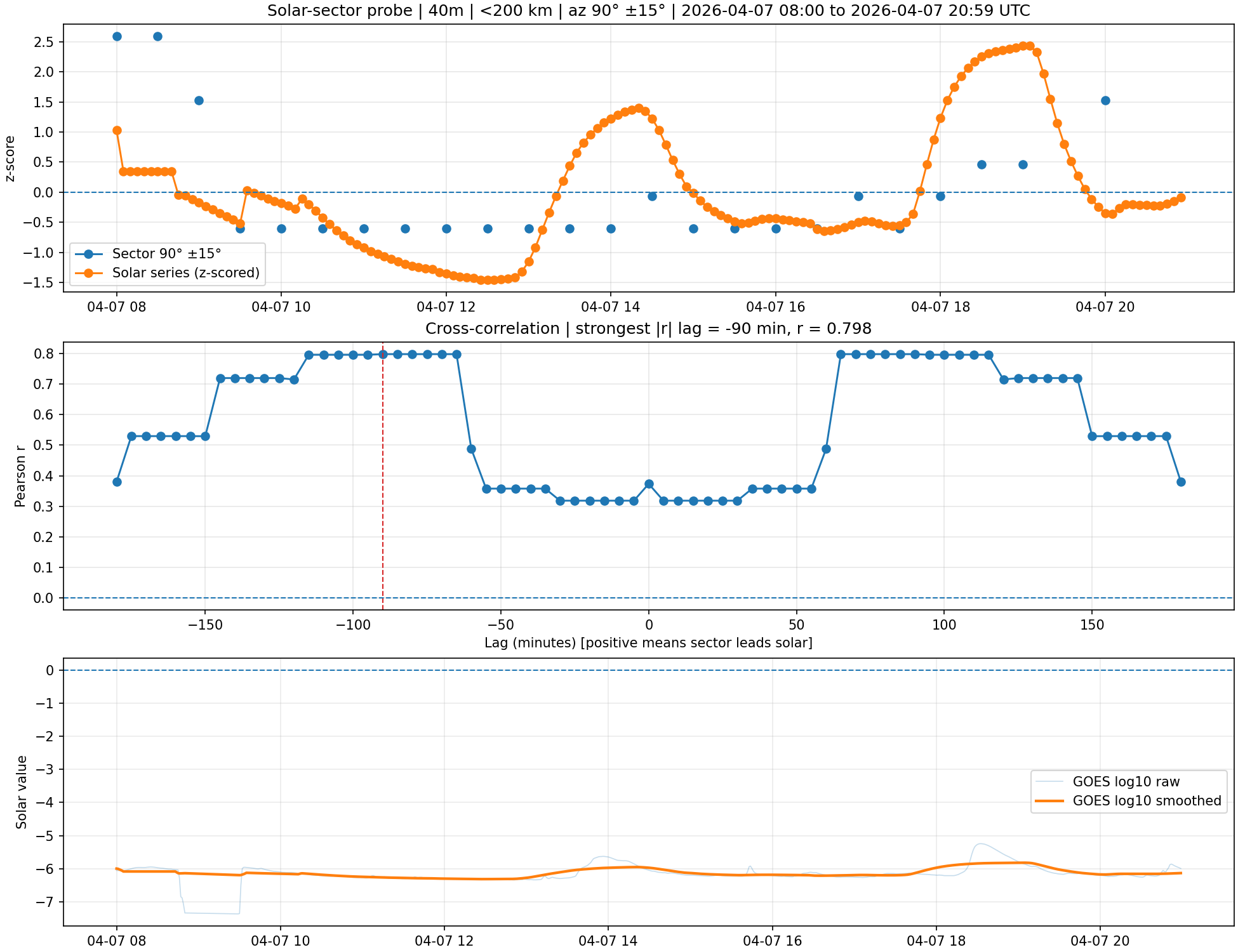
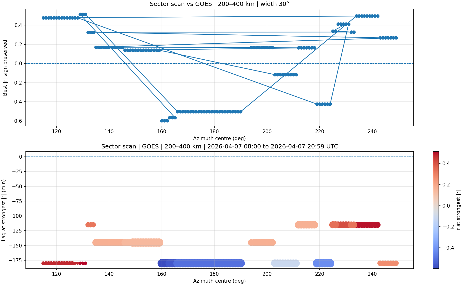
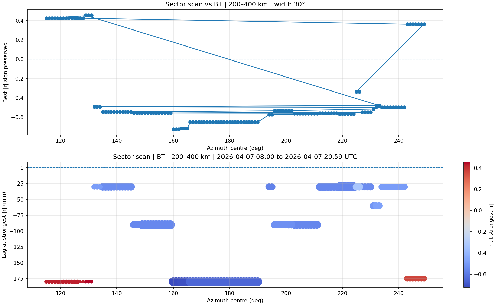
These are included as notebook-style supporting material. Some looked promising during testing, but none remained stable enough to support a clean solar-linked interpretation.

4. Receiver-mixing as the hidden cause of the ambiguity

Reducing the dataset from many reporters down to just 4 receivers did not reveal any hidden solar-linked behaviour. The distance-dependent structure remained, but no stable lag or alignment emerged.

Comparison view: Single receiver plot

Simplifying the geometry clarifies the signal — but does not reveal a hidden solar driver.

Taken together, these tests show that while correlations can be produced under many parameter choices, none remain stable under small changes in selection or method.

Why the solar and lag tests do not settle the mechanism

Different azimuth sectors would not necessarily be expected to share the same lag behaviour. A genuine externally driven response could plausibly appear with different delays in different directions, since each sector samples different propagation geometries and different ionospheric regions.

However, that does not remove the need for internal consistency within a given sector. In the present analysis, the inferred lag values remain highly sensitive to sector definition, smoothing choices, time-window choice, and tested solar parameter, and do not form a stable or repeatable pattern.

Interpretation

The most conservative reading is now also the strongest one: a real and repeatable distance-dependent offset structure exists, but simple correlation and lag methods do not identify a stable solar or geomagnetic driver for it.

The most plausible remaining explanation is propagation geometry rather than a single external driver. Different path lengths sample different combinations of takeoff angle, reflection height, hop structure, and ionospheric region. As those evolve through the day, the different path-length groups need not move together.

The experiment can be summarised simply: the ionosphere was “poked” It’s a highly advanced diagnostic technique. Very cutting edge. Involves staring at plots until they confess. , and it did indeed wobble — just not in any way that aligns with the obvious solar controls tested here.

Behaviour of this type has been described in the context of propagation-induced Doppler and ionospheric dynamics, but is not commonly examined at this level of resolution within narrowband amateur radio datasets.

What this means

What remains open

• Comparison with other bands
• ** Cross-band comparison: preliminary re-analysis of earlier 20 m data shows much weaker and less stable distance-dependent separation, consistent with increased path mixing and MUF-dependent variability on that band
• Detrending and alternative lag methods
• Comparison with ionosonde data (hmF2 / foF2) [Currently investigating]
• Whether a more controlled single-path or beacon-style dataset would isolate a cleaner physical observable