QSO Take-off Angles — M7SQI

What the viewer shows

This approach is geometry-rigorous but ionosphere-approximate. It infers plausible launch-angle regimes and probable hop structures for the QSOs actually observed; it does not reconstruct exact propagation paths. The model assumes approximately repeated, ground-touch F-mode hops and great-circle geometry. Unequal hops, ionospheric tilts, ducts, chordal paths, off-great-circle propagation, and full ray-tracing were not modelled. TOA is computed with atan2 and clamped to ≥0°; unusually shallow solutions are treated as candidate low-angle anomalies, not confirmed propagation modes.
NOTE: Work still in progress —

How the angles were calculated (ham-science summary)

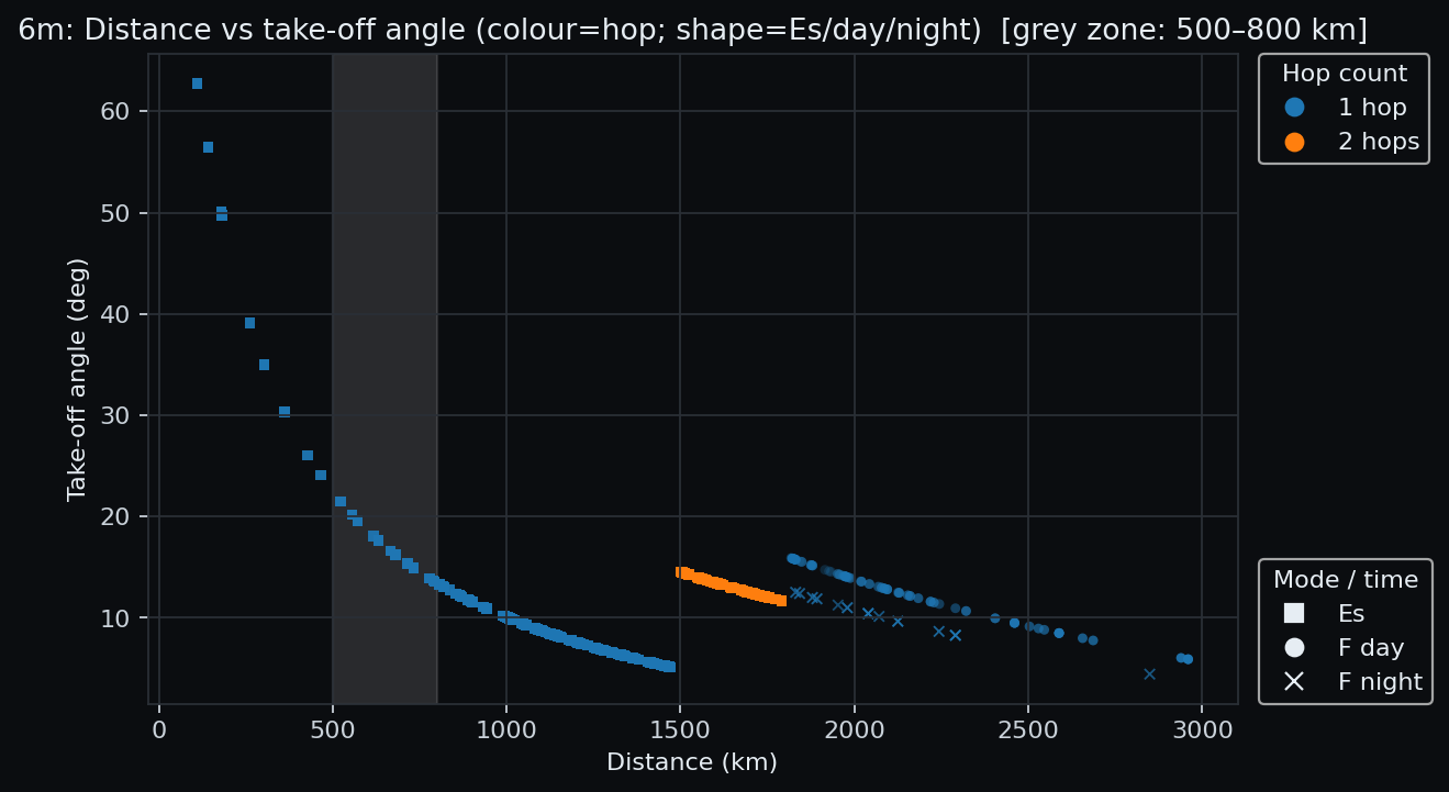
1. Per-band Es/F split. Short-range distance histograms were smoothed and a threshold was selected; values were then clamped to a sensible range. On 6 m a higher threshold was adopted, because paths there were typically Es.
2. F single-hop spacing (μ). The distance histograms exhibited a comb at multiples of an underlying hop length. A seed μ was estimated from that periodicity, refined by minimizing the spread of distance mod μ, and finally tuned by a short grid search per band and for day/night.
3. Heights. Virtual reflection heights of approximately 340 km (F, day), 280 km (F, night), and 110 km (Es) were used.
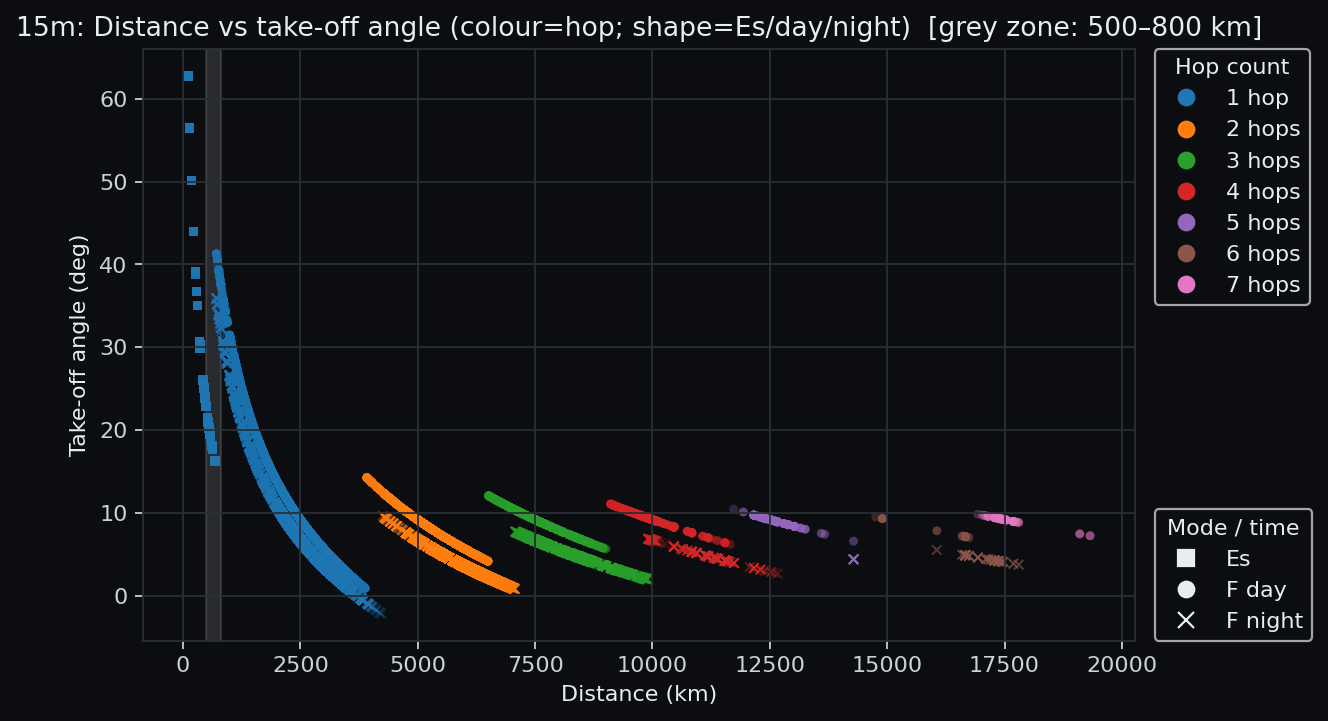
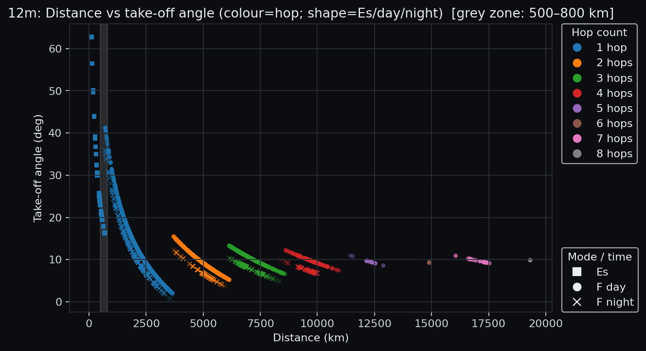
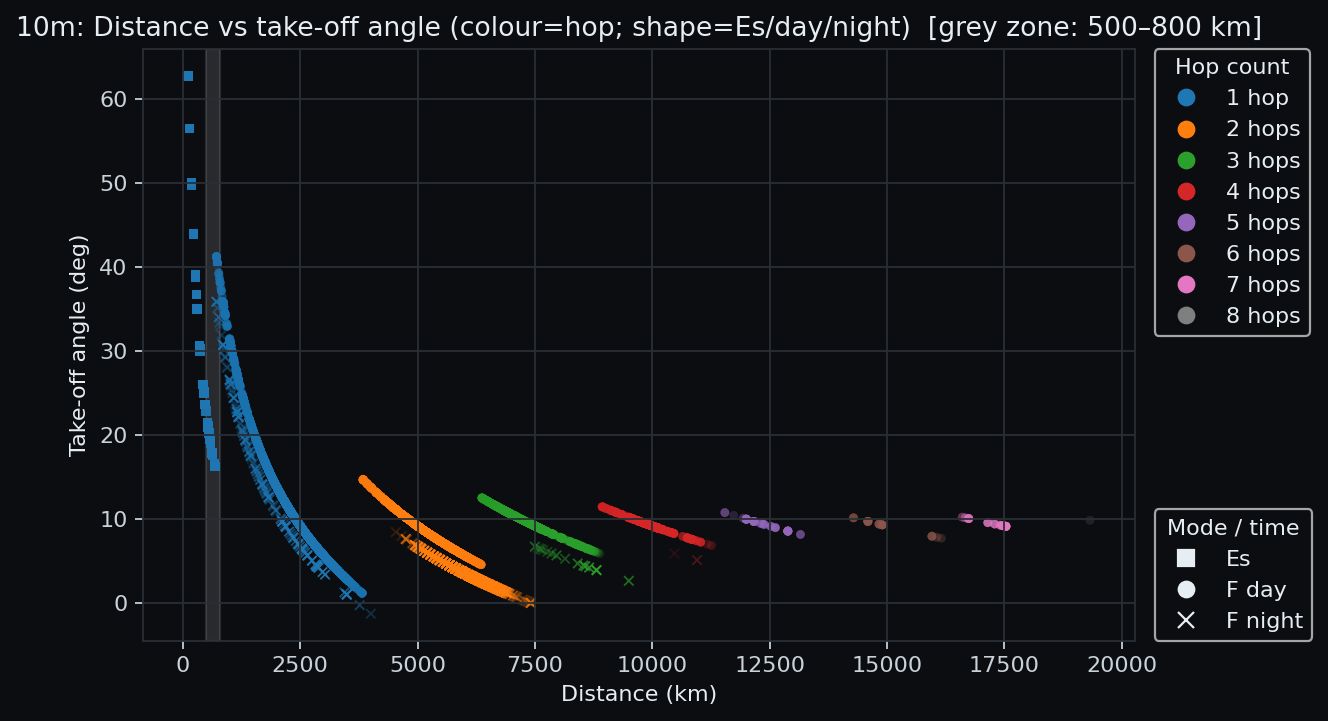
4. Hop count. For F-mode, n ≈ round(D/μ) was used with guards against sub-hop artefacts and unrealistic values, assuming ground-touch per hop. A maximum modelled hop count was imposed. Where a path reaches this model limit with very low hop-fit confidence, the reported hop count should not be interpreted literally: it indicates that the simple equal-hop model cannot provide a satisfactory conventional solution. Such paths may involve unequal hops, chordal propagation, ducting, or other complex long-haul geometry. For 6 m, multi-hop Es counts were optionally reported using a nominal Es hop length.
5. Geometry. The take-off angle was the elevation that reached one hop of D/n at the chosen virtual height on a spherical-Earth approximation. In code form: e = atan2(2h′, D/n) (in degrees). No path-loss modelling was applied—this was geometry only.

This approach is geometry-rigorous but ionosphere-approximate; it was appropriate for interpreting which angles were likely used by the QSOs actually made, assuming equally spaced, ground-touch F-mode hops (no tilts/ducts/chordal or full ray-tracing). TOA is computed with atan2 and clamped to ≥0°; values implying unphysically shallow geometry are flagged below.
NOTE: Work still in progress —

i) Very low inferred TOA values are flagged as possible chordal/ducted candidates:

• Possible chordal/ducted candidate: 4–6°
• Probable chordal/ducted candidate: <4°
• These flags indicate unusually shallow inferred geometry only; they do not prove chordal or ducted propagation.

The chordal/ducted flags above are deliberately narrow angle-based indicators. A value of False does not rule out complex or chordal propagation, particularly where the fitted hop count reaches the model maximum and the hop-fit confidence falls to zero.

ii) Factor in Greyline effects — Solar elevation at the QSO time for both endpoints:

• Use any SPA lib (e.g., astral, pysolar, ephem).
• Get sun_alt_tx and sun_alt_rx in degrees and tag:
  • Dual greyline (strict): |alt| ≤ 6° at both ends
  • Single-end greyline (strict): exactly one end |alt| ≤ 6°
  • Near-greyline (loose): repeat with 12°
  • (Optional) Sample points along the great-circle; if >50% have |alt| ≤ 6°, tag as a path “terminator-skimmer”.

Reading the results

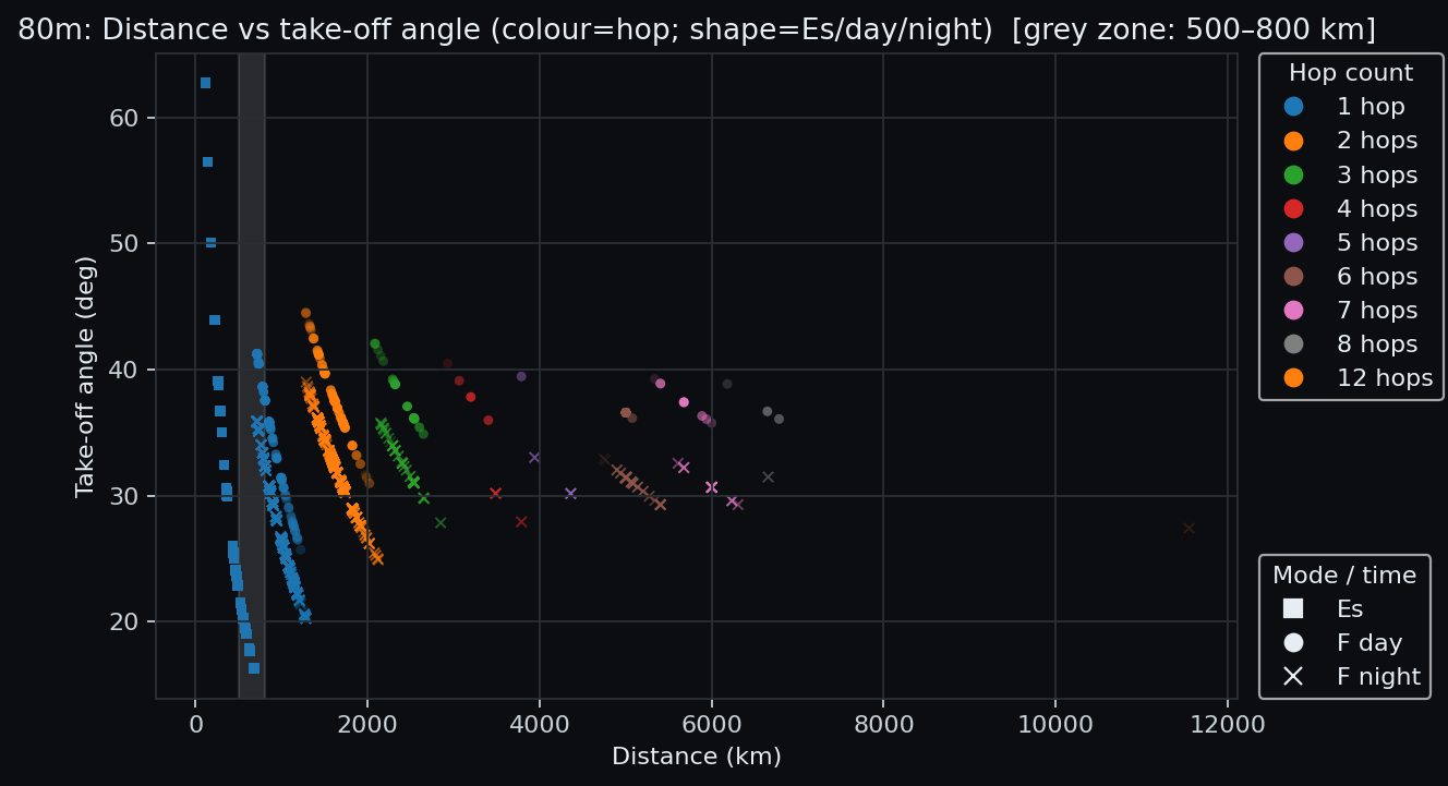
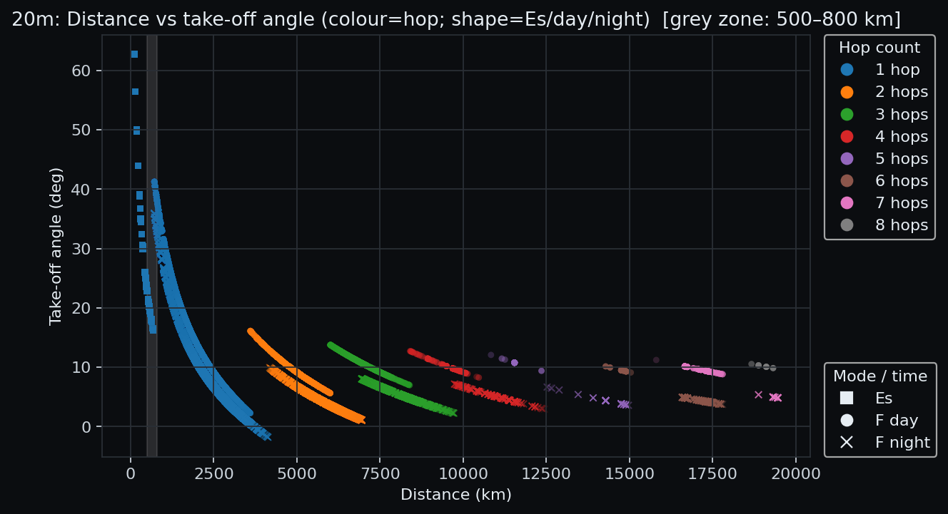
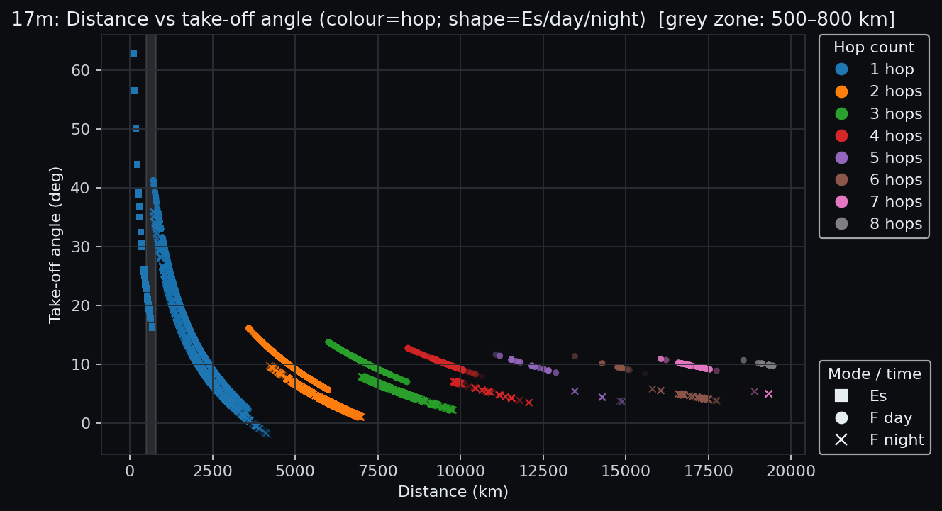
• Typical DX angles. On 20/17/15 m, long paths commonly clustered in the low-angle regime (roughly single-digit to low-teens degrees).
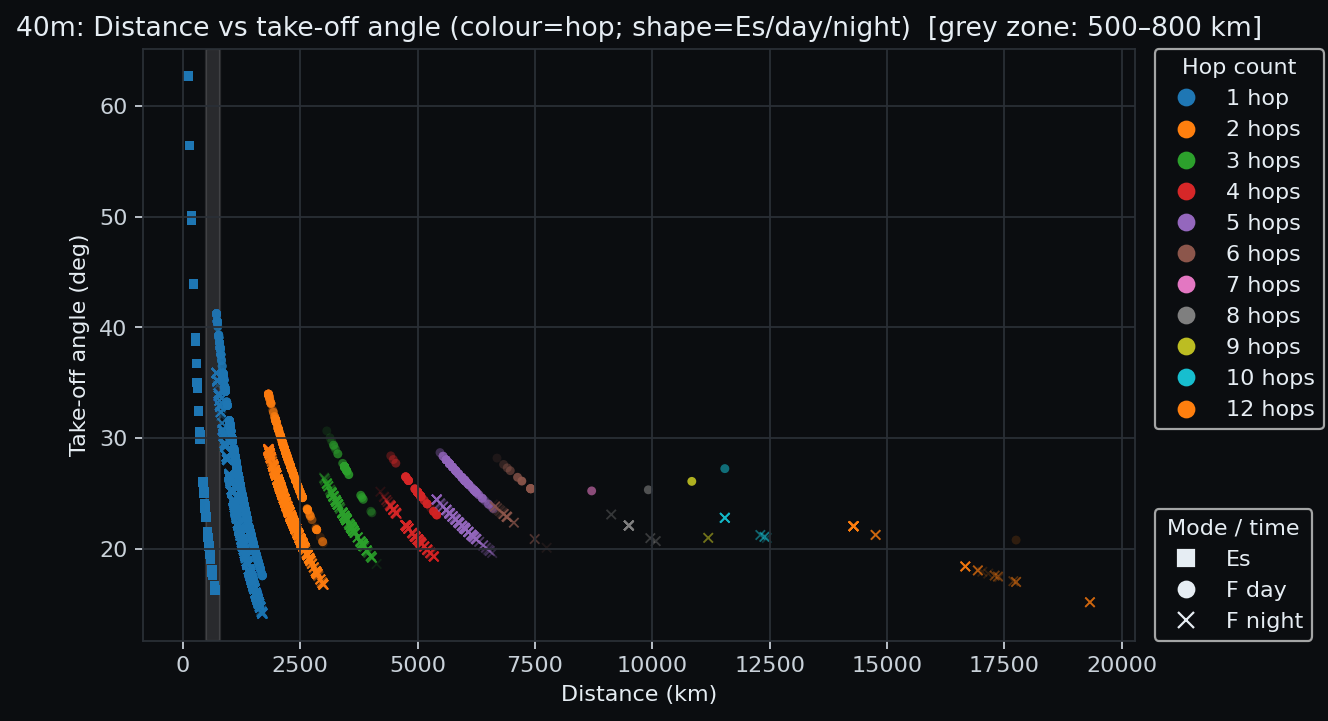
• Why 40 m usually looked “shorter-hop”. Higher average launch angles (plus daytime D-layer absorption) generally shortened per-hop ground ranges compared with 20/17/15 m. A small number of extreme 16–19 Mm paths were also observed; these sit beyond the region where the simple equal-hop model gives a confident physical hop count.
• 6 m was Es-dominated. At mid-latitudes, F2 at 50 MHz was rare; multi-hop Es and, seasonally, TEP were more typical drivers of long 6 m paths.
• Antenna Analysis - I ran some antenna modelling analysis to try and validate the data here. The Results can be seen on this page

Limits & uncertainty

Single virtual heights, equal hop lengths, and great-circle propagation were assumed; off-great-circle tilts, ducts and full ray-tracing were not modelled. Median take-off angles were expected to carry a small systematic uncertainty (a few degrees), which was acceptable for band-to-band comparisons. Clearly implausible records and known artefacts were excluded, but genuine extreme-distance observations were retained even where the simple hop model could not assign them a high-confidence conventional solution.

Where the ionosphere numbers came from

The ionosphere was measured continuously by ground ionosondes and satellites. Useful sources included:

• GIRO / DIDBase: global ionosonde network with ionogram-derived parameters (foE, foF1, foF2, hmF2, etc.). DIDBase and the GAMBIT nowcast.
• NOAA NCEI Mirrion: near real-time plots of foF2, hmF2, and foEs, plus the World Data Service archive. Mirrion real-time · NCEI ionosphere portal.
• Reference models: the International Reference Ionosphere (IRI) provided monthly climatology of electron density and F-region parameters. IRI · NASA CCMC IRI.
• Spaceborne profiles: COSMIC-2 radio-occultation delivered global electron-density profiles used for validation and nowcasting. COSMIC-2 data.
• Regional examples: UK RAL/Chilton and Belgium RMI/Dourbes maintained long time series of ionosonde measurements. Chilton / UKSSDC · RMI Dourbes.

These references underpinned the typical heights and the day/night behaviour used in the simple geometric model presented above.